Part A: The Power of Diffusion Models!

Overview

In this part of the project, I play around with the pre-trained DeepFloyd IF diffusion model, which was obtained from Hugging Face. I worked on implementing diffusion sampling loops and use that along with computed text embeddings for tasks such as inpainting, creating anagrams, and creating hybrid images.

Sampling from the Model

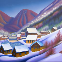
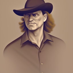
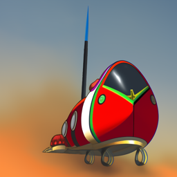
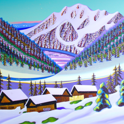
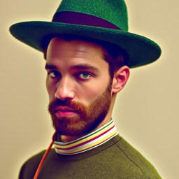
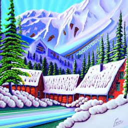
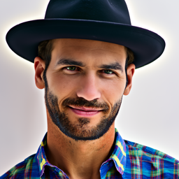
Below are some samples from the model using various prompts and number of inference steps and upsampled from 64 x 64 to 256 x 256 using a random seed of 1142024. The text prompts used for these were "an oil painting of a snowy mountain village", "a man wearing a hat", and "a rocket ship".

As we can see above, the number of the quality of the output image is postively correlated with the inference steps used in the sampling. There was siginificant improvement for all three images from 10 to 20 inference steps. The most improvement was seen in the image of the man wearing a hat from 20 to 40 inference steps.

Implementing the Forward Process

The first part of implmenting the sampling loop is implementing the forward noising process. Given a clean image \(x_0\), we add noise to the image in the following way: $$q(x_t|x_0) = \mathcal{N}(x_t; \sqrt{\bar{\alpha}}x_0, (1 - \bar{\alpha_t})\mathbf{I})$$ which is equivalent to, $$x_t = \sqrt{\bar{\alpha}}x_0 + \sqrt{1 - \bar{\alpha}\epsilon}, \epsilon ~ \mathcal{N}(0, 1)$$ Each of \(\bar{\alpha}\) is provided from the model. Here are some examples of the foward process being applied to an imagine of the Campanile on Berkeley campus:

Classical Denoising

Below I attempt a naive method of denoising which involves applying a Gaussian filter on each noisy image. This evidently is not a great solution and its effectiveness decreases as the amount of noise applied increases.

One Step Denoising

We can more effictively denoise our images by passing them and a time step t through our trained UNet, which can recover Gaussian noise from our image. We can then remove this predicted noise from the image and get something close to our original image. The text prompt used for this denoising was "a high quality photo". Below are the outputs of doing this:

We can see that as t gets larger, our one step denoising results in an image that looks roughly good, but further away from the orignal image of the Campanile.

Iterative Denoising

Since one step denosing performs worse as the amount of noise in the image increases, we can try iteratively denoising our image starting at timestep \(T = 1000\). Since taking individual steps until we reach \(t = 0\) would be very expensive, we taking steps with a stride of 30. For a timestep \(t' \lt t\), we denoise image in the following manner: $$x_{t'} = \frac{\sqrt{\bar{\alpha_{t'}}}\beta_t}{1 - \bar{\alpha_t}}x_0 + \frac{\sqrt{\alpha_t}(1 - \bar{\alpha_{t'}})}{1 - \bar{\alpha_t}} x_t + v_{\sigma} $$ where, \(\bar{\alpha_t}\) is defined by the model, \(\alpha_t = \frac{\bar{\alpha_t}}{\bar{\alpha_{t'}}}\), \(\beta_t = 1 - \alpha_t\), and \(v_{\sigma}\) is random noise predicted by the model. Below are images as the appear throughout the denoising process as well as the final product compared to the one step denoising, the gaussian blurring, and the original image.

Diffusion Model Sampling

We can also use this iterative denoising process to create images from scratch. We do this by starting out with an image of pure noise and and iteratively denoising from there. The prompt used here was "a high quality photo".

Classifier-Free Guidance

As we can see above, the images produced are not very good. We can remedy this with a technique known as classifier-free guidance (CFG), in which we predict a conditional and unconditional noise estimate, denoted \(\epsilon_c\) and \(\epsilon_u\) respectively. Then we compute our new noise estimate: \(\epsilon = \epsilon_u + \gamma(\epsilon_c - \epsilon_u)\), where \(\gamma \gt 1\). For the below sampled images, \(\gamma = 7\), the text prompt for conditional guidance is "a high quality photo", and the text prompt for the unconditional guidance is "".

Image-to-Image Translation

Now using CFG, we can do image-to-image translation, where we start off by adding some noise to our image, and iteratively force it back onto the manifold of natural images. I did this on various images, starting from various noise levels \(i\), where \(i\) is the number of strided time steps away we are away from our clean image at timestep \(t = 0\). The effect we will see is that when \(i\) starts off low, the result will be far from the original image, but as \(i\) increases, the result get closer and closer to the original. Through this process we can see some pretty interesting images.

Editing Web Images and Hand Drawn Images

The above process can also be performed on non-realistic or hand drawn images, which produces cool intermediate images as the model attempts to force the image onto the manifold of natural images.

Inpainting

We can also use this technique to do inpainting. We define a region of our image that we want to regenerate via a binary mask. Then we go through the deniosing process, but as the last step of every iteration, we force \(x_t\) to have the same pixels as the original image noised at the current value outside of the designated mask. Formally, $$x_{t} = \mathbf{mask} * x_t + (1 - \mathbf{mask}) * forward(x_{original}, t)$$ Below are some images that this was performed on:

Text Conditional Image-to-Image Translation

Prompt: "a rocket ship"

Prompt: "a photo of a man"

Prompt: "a photo of a dog"

Visual Anagrams

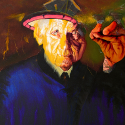
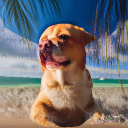
We can also use CFG to create optical illusions. In this section, I show anagrams that I created. To do this we can predict the noise for two separate text prompts and average them together for each iteration. For the conditional noise, unconditional noise, and predicted variance, values were predicted with one prompt on our image normally, and then the image is rotated \(180^{\circ}\) and then values are predicted with this flipped image and the other prompt. The predicted noise is also flipped before averaging. Below are some of the anagrams that were created. I also passed the results through an upsampler provided in the downloaded model.

Prompts: "an oil painting of an old man" + " an oil painting of people around a campfire"
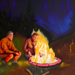
Prompts: "an oil painting of a snowy mountain village" + "a photo of the amalfi coast"
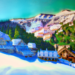
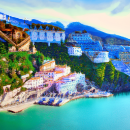
Prompts: "a photo of a man" + "a photo of a dog"

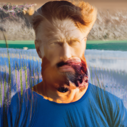
Hybrid Images

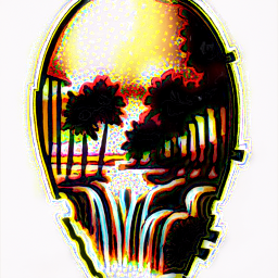
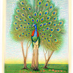
In a similar way to making anagrams, we can make hybrid images. We still predict the noise of two different prompts, but we initially pass the original image into the model twice, and then apply a low pass filter onto one set of predicted noises and variance and a high pass filter onto the other set of predicted noises and variance. Through this process, we get a hybrid image that looks like one thing from afar where low frequencies are dominant, and another thing up close, where high frequencies are dominant. Below are some samples that I created as well as the upsampled version:

Prompts: "a lithograph of a skull" + "a lithograph of waterfalls"
Prompts: "a lithograph of a turtle" + "a lithograph of flowers"
Prompts: "a lithograph of a trees" + "a lithograph of a peacock"

Part B: Diffusion Models from Scratch!

Overview

In this part of the project, I work on creating a diffusion model from scratch and implement it on the MNIST dataset of hand written numbers.

Training a Single-Step Denoising UNet

To do this I first implemented a UNet that will act as a simple one-step denoiser. The goal is that when Given a noisy image \(z\), the denoiser \(D_{\theta}\) will map \(z\) to the clean image \(x\). Here we optimize over an L2 loss: $$L = \mathbb{E}_{z,x}||D_{\theta}(z) - x||^2 $$ Below is a schematic of the implemented UNet:

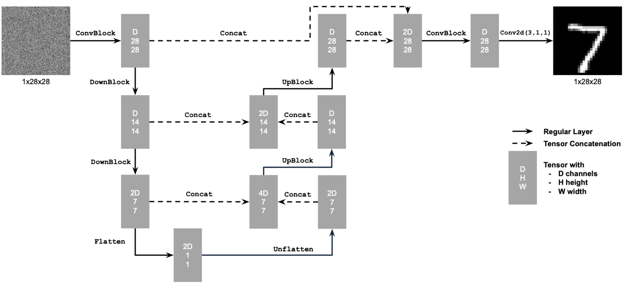
The above diagram uses some standard tensor operations which defined as following:

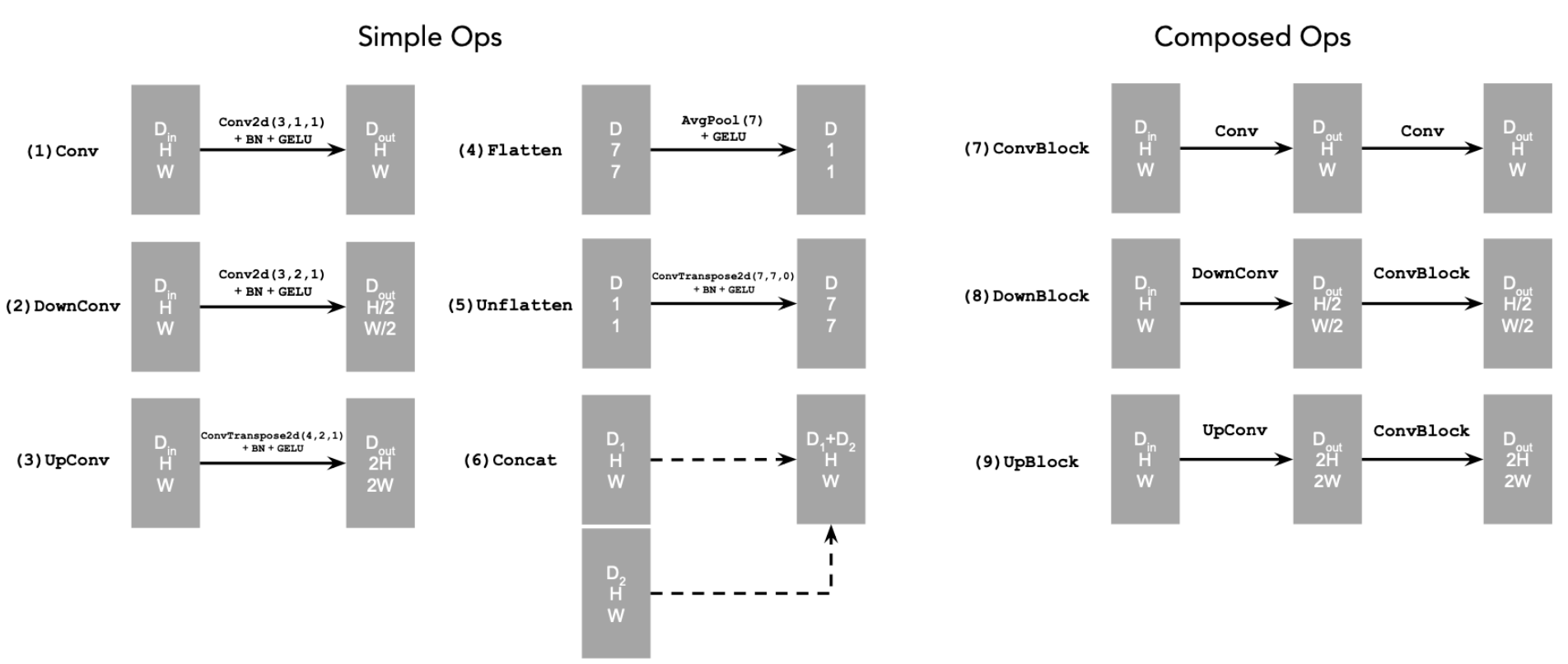
where,

Conv2d(kernel_size, stride, padding) is torch.nn.Conv2d()

BN is torch.nn.BatchNorm2d()

GELU is torch.nn.GELU()

ConvTranspose2d(kernel_size, stride, padding) is torch.nn.ConvTranspose2d()

AvgPool(kernel_size) is torch.nn.AvgPool2d()

D is the number of hidden channels and is a hyperparameter

I implemented this model and then trained it on a modified version of the MNIST dataset where noise was injected into each image. For each clean image \(x\), a noisy image \(z\) was created in the following manner: $$z = x + \sigma\epsilon, \epsilon ~ \mathcal{N}(0, I)$$ Below is a visualization of several images in the MNIST dataset with various levels of noise added, which is controlled by \(\sigma\):

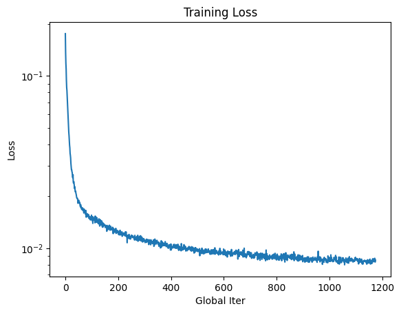
The following loss plot shows the progression of the model as it was trained for 5 epochs. Note that the y-axis has a logarithmic scale.

In-Distribution Testing

As the model was training, I saved the weights after the first and fifth epochs and used them to test the denoising capabilites of my model at each of these points. I first tried them on in-distribution images in which \(\sigma = 0.5\). Here are the results:

Out-of-Distribution Testing

Additionally I tested this model's efficacy for images outside of its trianing distribution with noise levels that varied from \(\sigma = 0.5\). In total I tried it with \(\sigma \in [0.0, 0.2, 0.4, 0.5, 0.6, 0.8, 1.0]\). As we might expect, the model is able to perform decent denoising on images that have \(\sigma \lt 0.5\) but struggles more with images that have \(\sigma \gt 0.5\) Here are the results at epochs 1 and 5:

Time-Conditioned UNet

In order to do iterative denoising, we need to condition our UNet on our timesteps. We do this by adding fully connected layers to the UNet in the following manner:

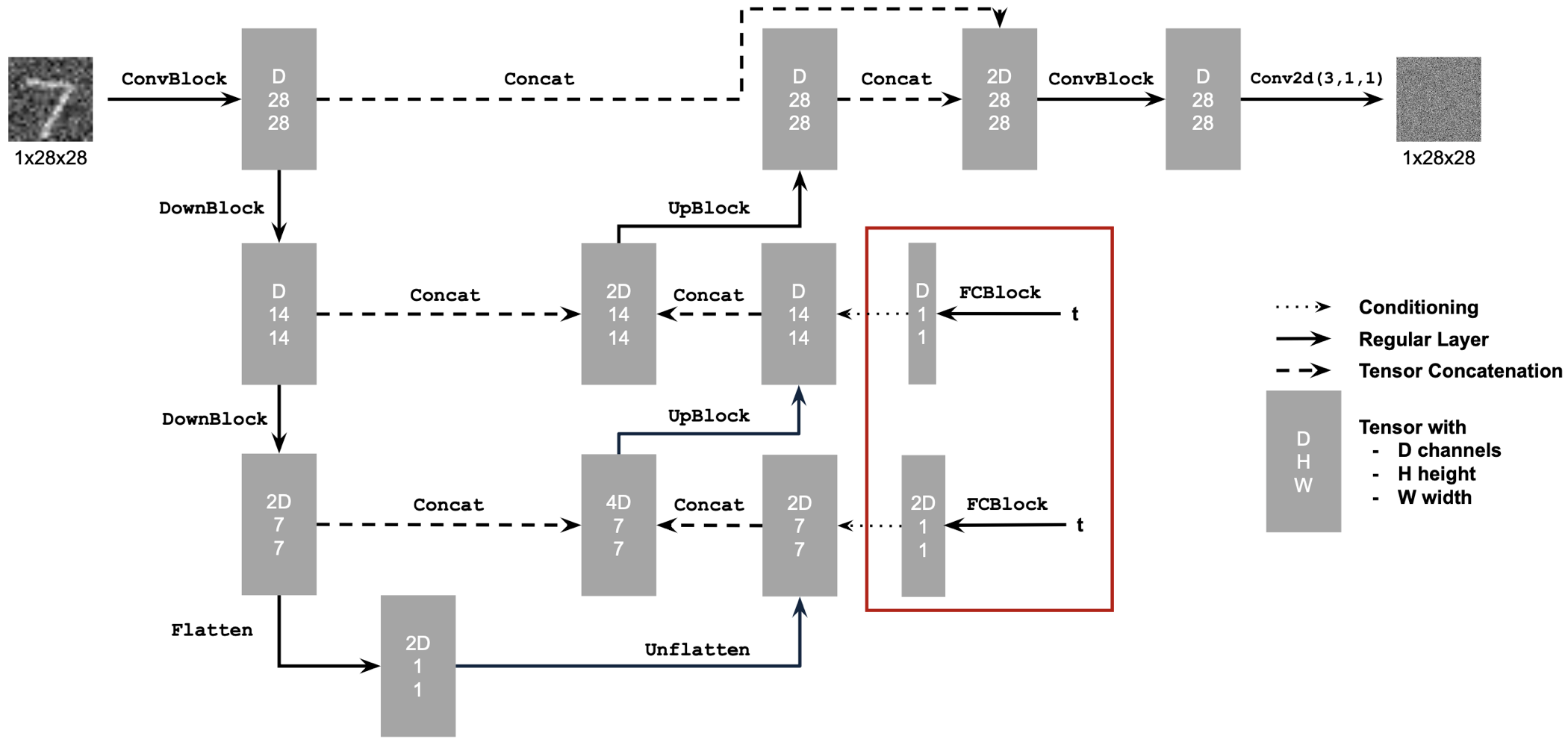
The FC block is defined in the following manner:

where Linear(F_in, F_out) is implemented via torch.nn.Linear().

Additionally we do the following:

Define a list of \(\beta\)'s starting at \(\beta_0 = 0.0001\) and ends at \(\beta_T = \beta_{300} = 0.2\) with an even spacing of values in between.

\(\alpha_t = 1 - \beta_t\)

\(\bar{\alpha_t} = \prod_{s=1}^{t} \alpha_{t}\)

Additionally, we now optimize over an L2 loss of the noise as opposed to the image pixel values. Note that these are mathematically equivalent. $$L = \mathbb{E}_{\epsilon, x_0, t}||\epsilon_{\theta}(x_t, t) - \epsilon||^2$$

The model was trained according to the following algorithm:

This time-conditioned UNet was trained for 20 epochs and the training loss graph looked like the following:

Next sampling of this model was done with the weights of the model at 5 and 20 epochs. The sampling was done according to the following algorithm:

Below are some the results from this sampling. As we can see, the time conditioning has significantly improved our results, but there is still some room for imporvement.

Class-Conditioned UNet

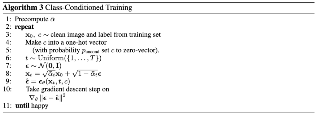
Similar to what we did in CFG, we can improve the results of our model if we do some class conditioning. This was implemented by adding two more fully connected layers that took in a one-hot vector describing the class of the digit we are trying to denoise. A dropout of this class conditioning was implemented as well where 10% of the time the class conditioning vector \(c\) was dropped. The training algorithm for the class-conditioned UNet looked like the following:

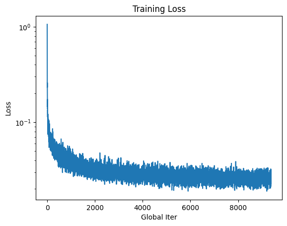
The training loss of this model over 20 epochs is as follows:

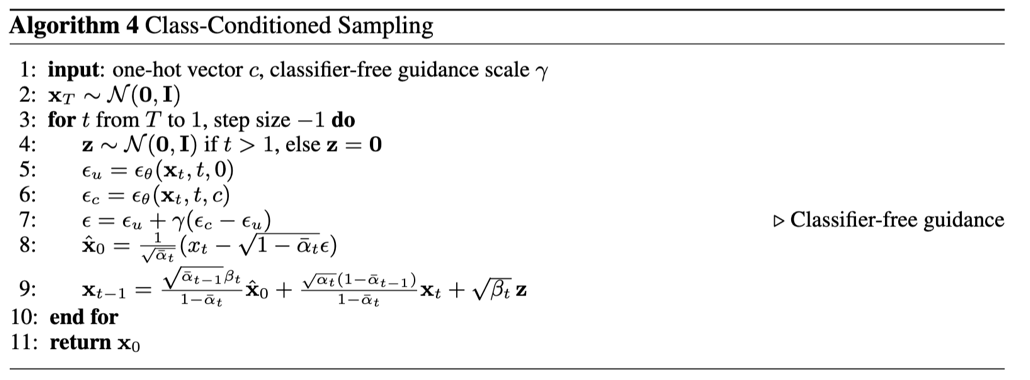
The following algorithm was used to sample from the model at 5 and 20 epochs:

Here are some the results from this sampling: