Part A: Image Warping and Mosaics

Overview

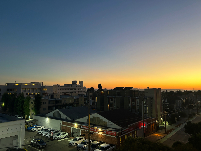
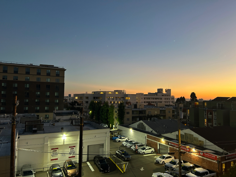
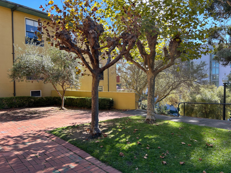
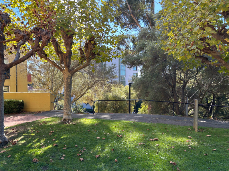
This project furthers the exploration of image warping through computing homographies between images and blending them to create a mosaic. The resulting image provides a greater perspective view than the original images. In this first part of the project, I implement a way to warp and moasic images given manually defined correpsondences on each image.

Capturing Images

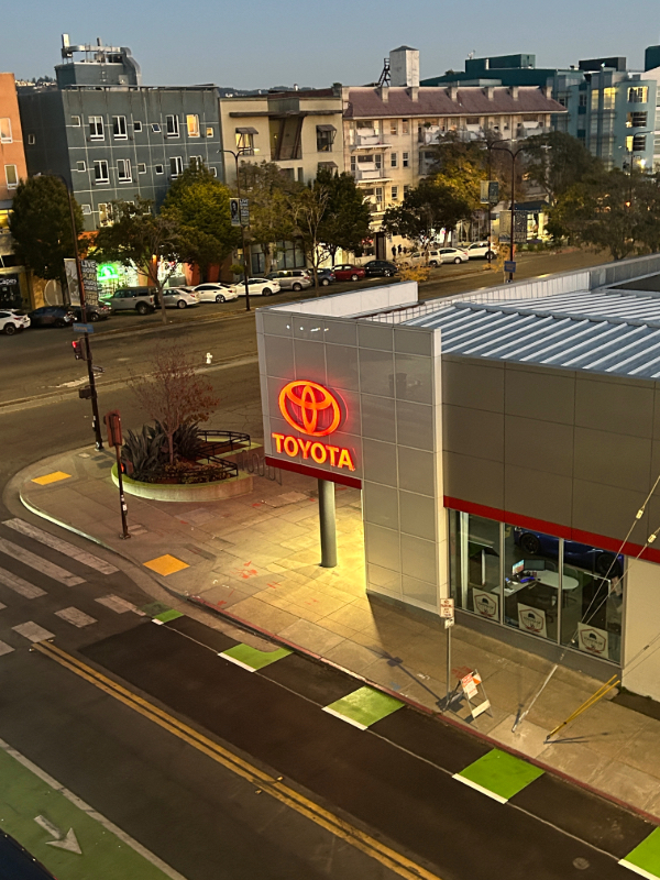
Here are some of the images that I used for this project:

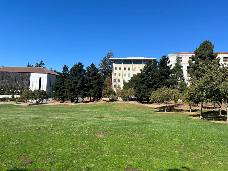
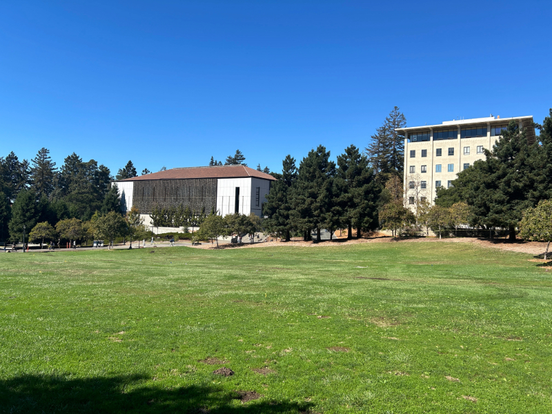
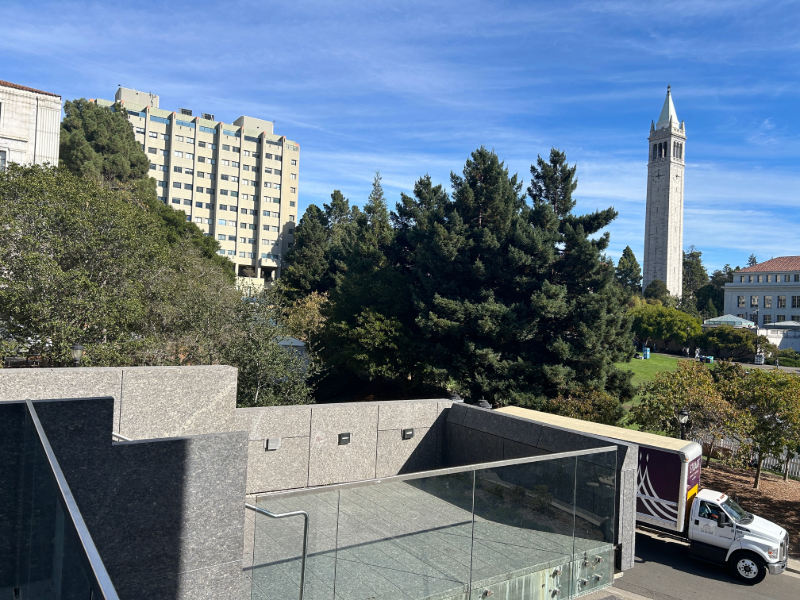
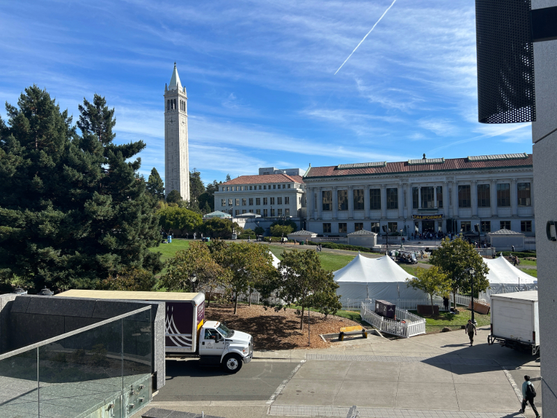
Recovering Homographies

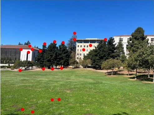
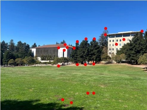
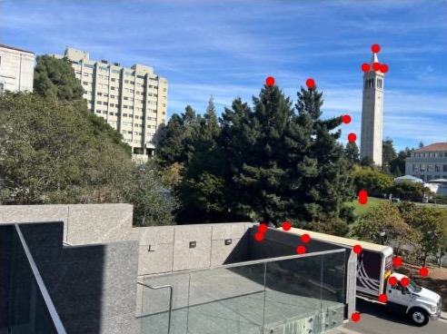
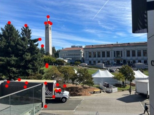
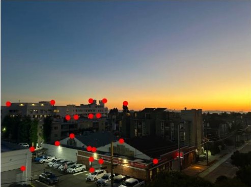
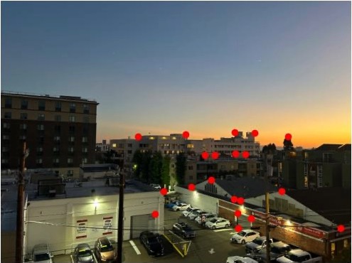
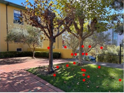
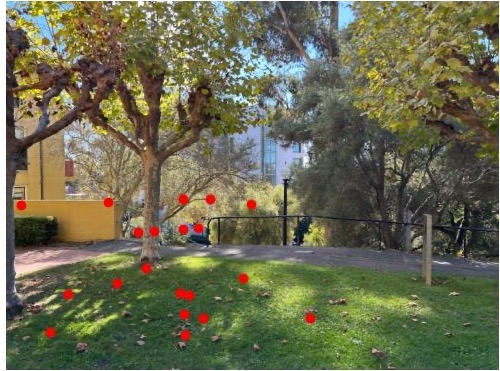
In order to recover the homographies between each of the images, I first manually defined correspondences for each pair of images. Here are the points that were defined for some of the above images.

With these points, it is now possible to recover the projective transformation between the two images. This transformation will be of the following form:

$$ \begin{bmatrix} a & b & c \\ d & e & f \\ g & h & 1 \end{bmatrix} \begin{bmatrix} x_1 \\ y_1 \\ 1 \end{bmatrix} = \begin{bmatrix} wx_2 \\ wy_2 \\ w \end{bmatrix}$$

We can then rewrite this matrix-vector equation to solve for unknown values in the matrix:

$$ \begin{bmatrix} x_1 & y_1 & 1 & 0 & 0 & 0 & -x_1x_2 & -y_1x_2 \\ 0 & 0 & 0 & x_2 & y_2 & 1 & -x_1y_2 & -y_1y_2 \end{bmatrix} \begin{bmatrix} a \\ b \\ c \\ d \\ e \\ f \\ g \\ h \end{bmatrix} = \begin{bmatrix} x_2 \\ y_2 \end{bmatrix}$$

So from here, we can vetically/horizontally stack the values of our correspondence points into the matrix and result vector in the above system. Now notice we have an overconstrained system and we can use Least Squares to solve. This is beneficial as it will work to minimize any noise introduced due to slightly inaccurate selection of correspondence points.

Now that we have the projective transformation, we can apply this matrix onto the points of one image to get the image warped to the perspective of the other image.

Image Rectification

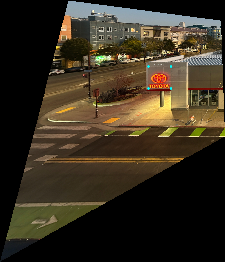
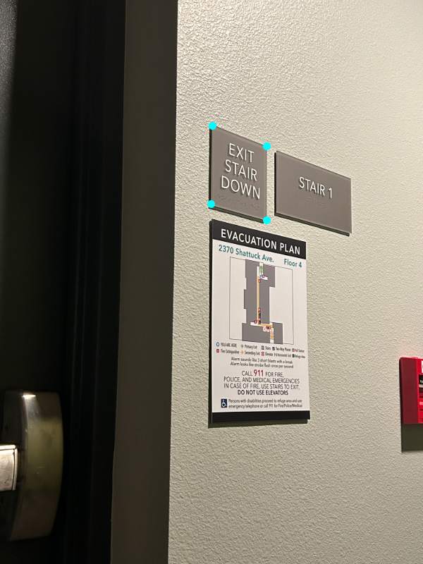
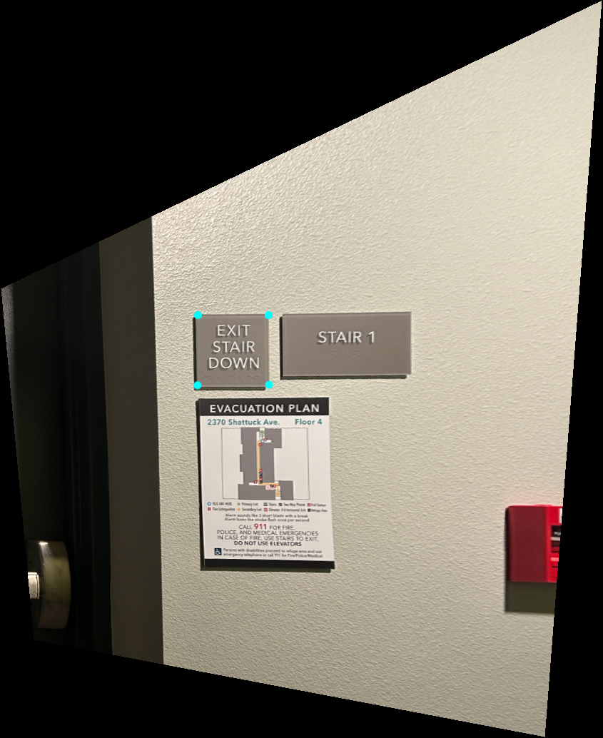
One cool thing we can do with homographies is "rectify" images. Given an image and a known perspective we want to view it from, we can transform the image to that perspective to "rectify" it. This was done capturing images with objects that are known to squares and then computing the homography between image and the coordinates of a square with some side length \(d\): \([0, 0], [0, d], [d, d], [d, 0]\). This was performed on the image of the Toyota dealership and a image I took in my apartmnet's hallway.

Blending Images

After we've warped one image to the perspective of the other, the final step in creating our mosaic is to blend them. After expanding each image to include all pixels in the bounding box of our final mosaic, I computed a distance transform, calculating the Euclidean distance from every pixel on the image to the closest black background pixel. Below are the visualizations of these distance transforms for the glade images:

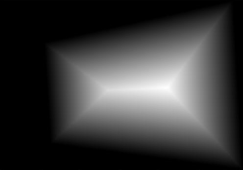
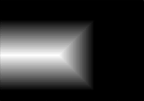
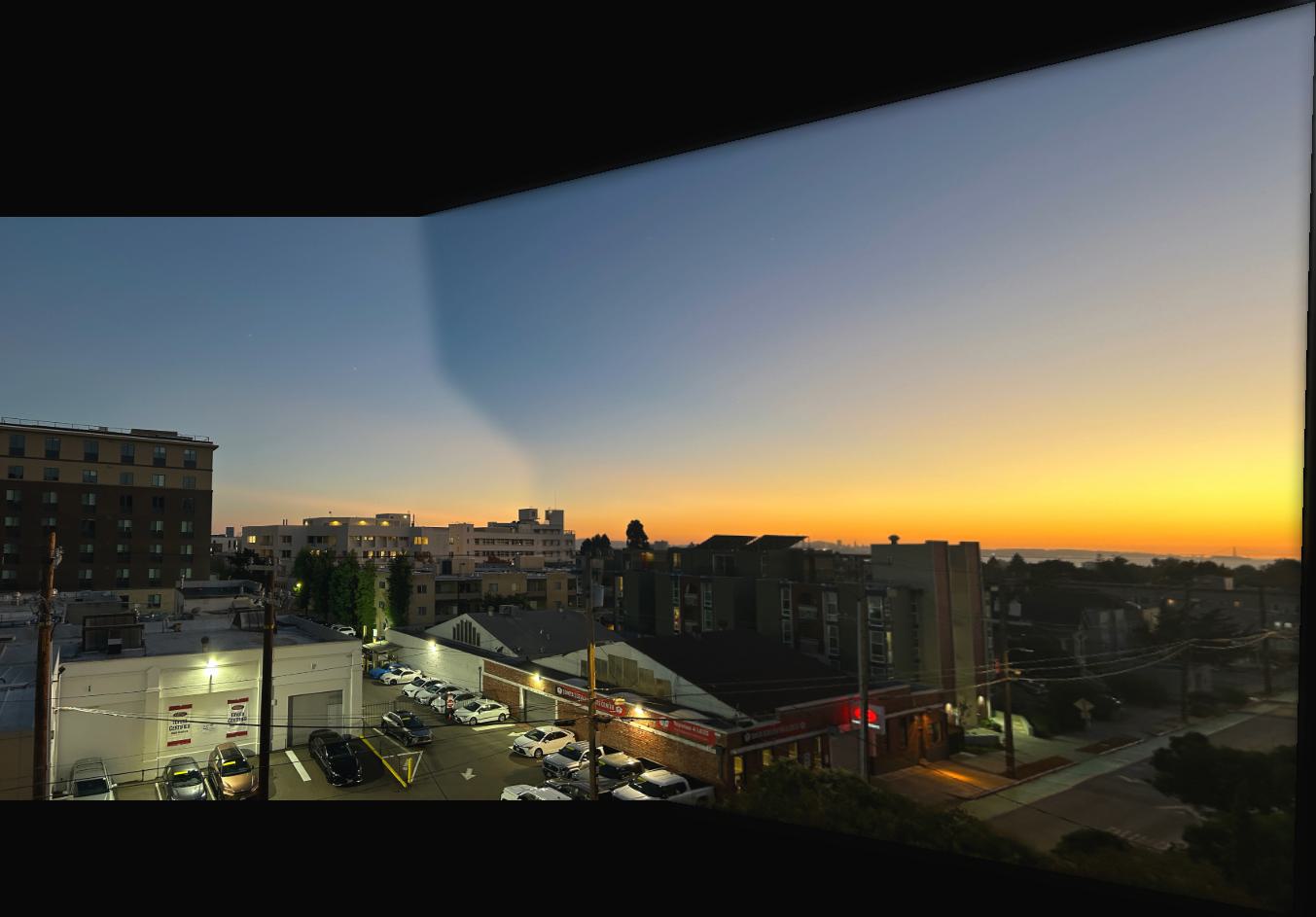
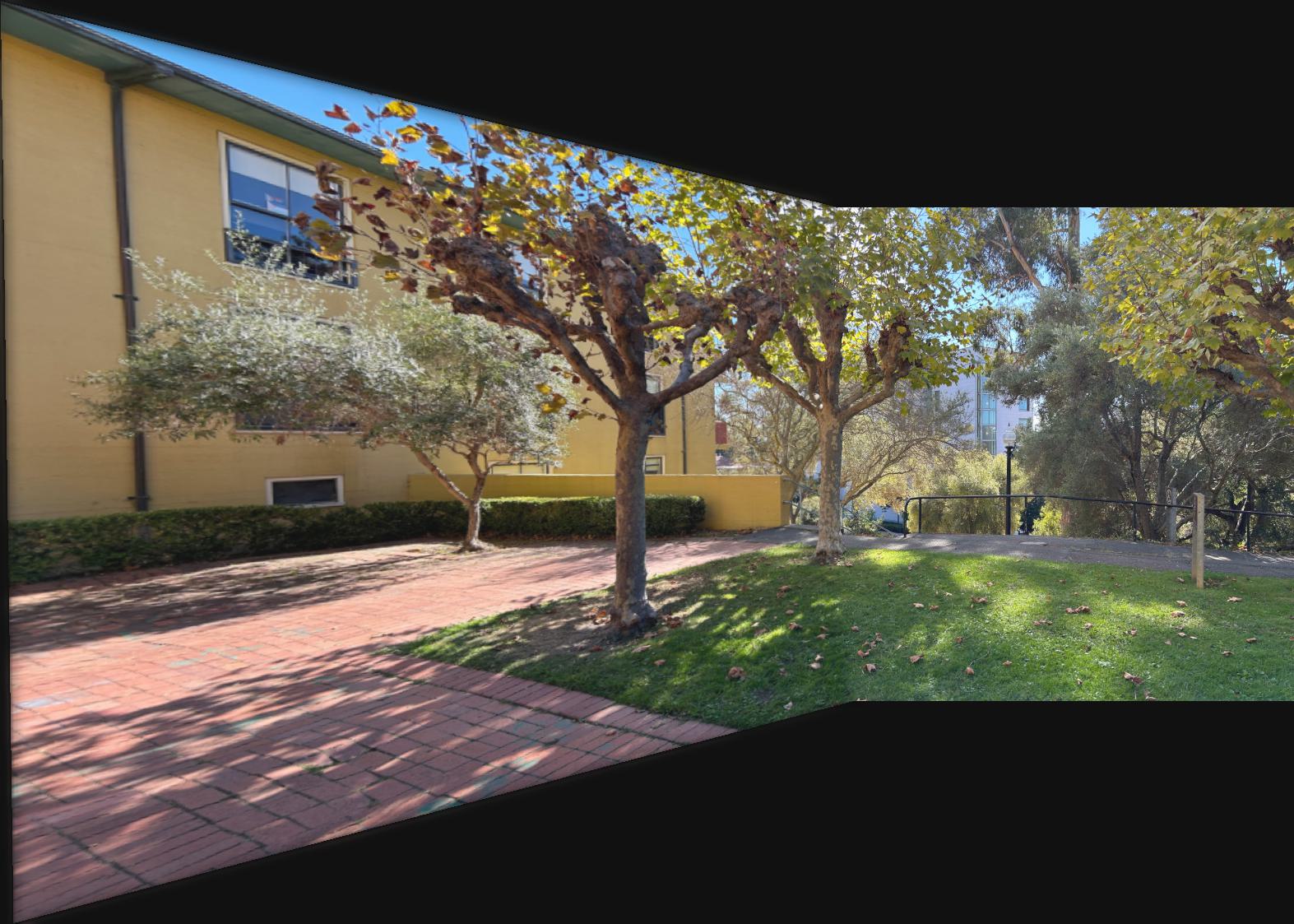
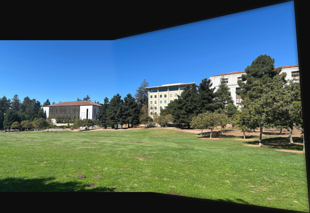
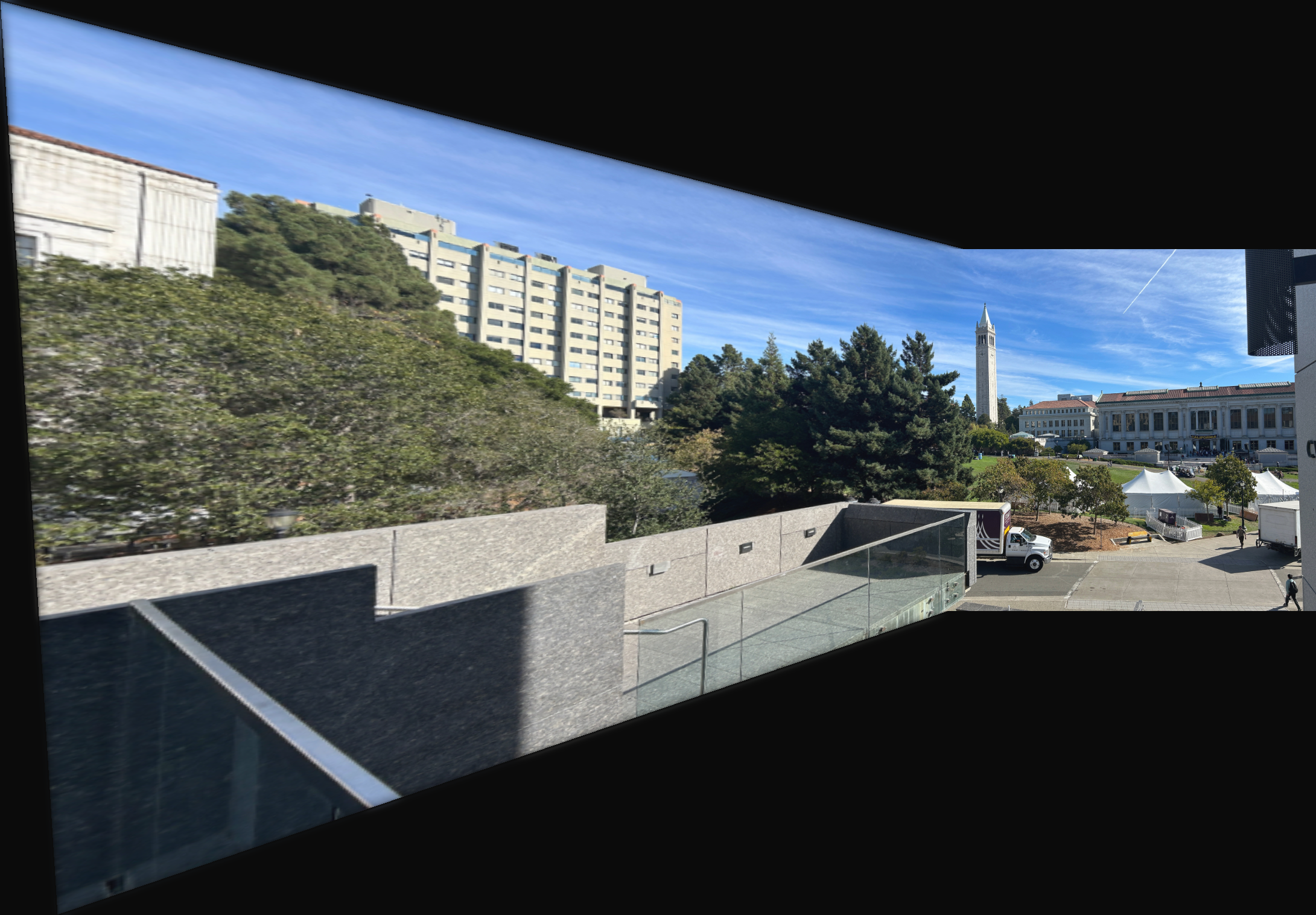
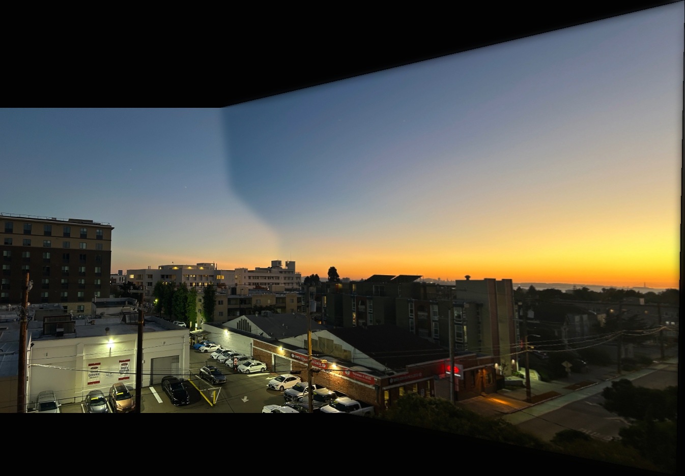
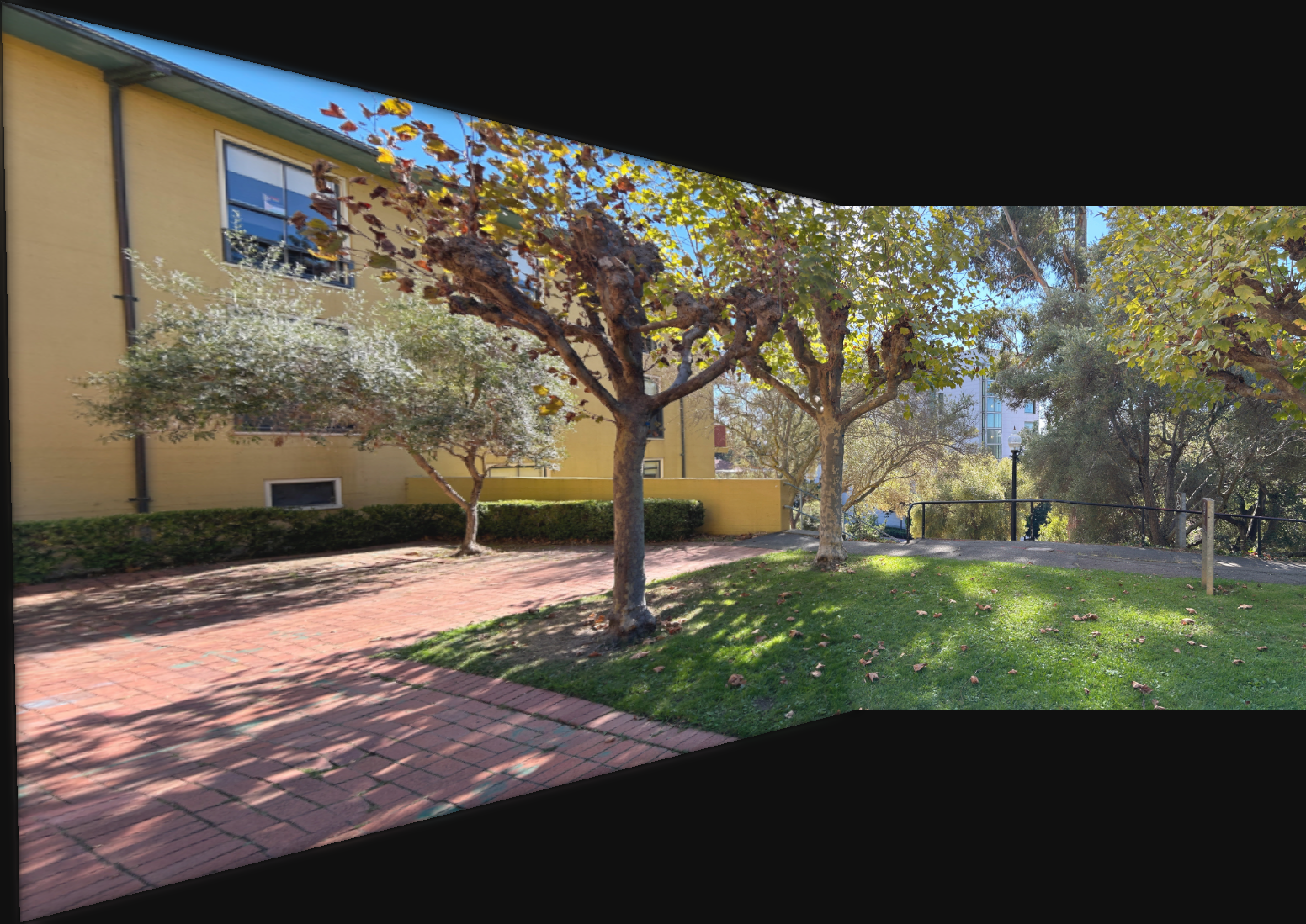
These transforms were then used to create masks that would be used to the blend the images. The blending technique used was two-band blending, where a two-level Laplacian stack was created and each frequecy level was blended independently. Some of the mosaics still have some artifcats where you can see that it is a stitching of two images. This was due to my iPhone camera changing the relative brightness in the images as it was rotated. Ideally, this brightness change would not have been present, but ultimately it did not affect the quality of the images too much. Below are the final results of the blending:

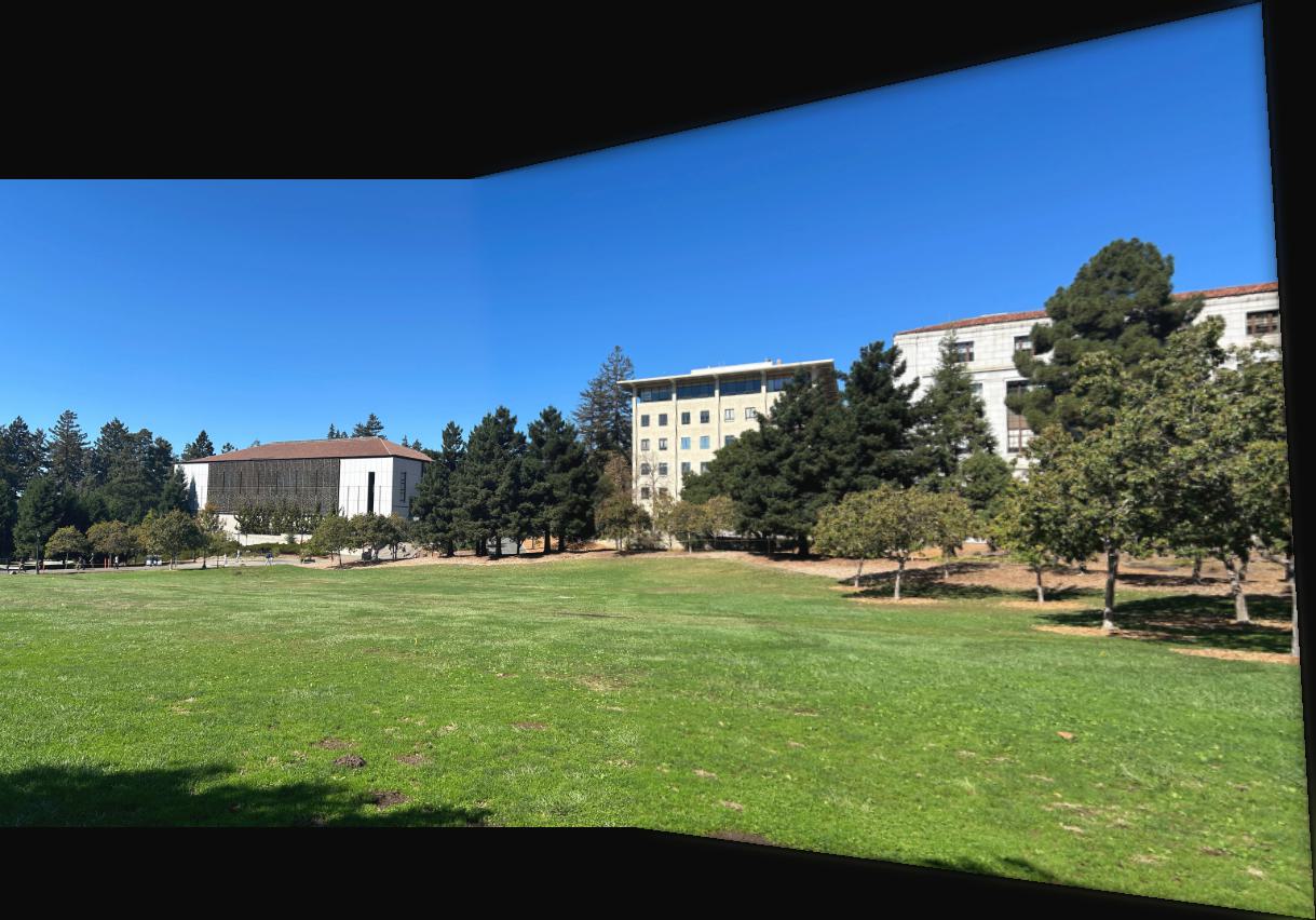
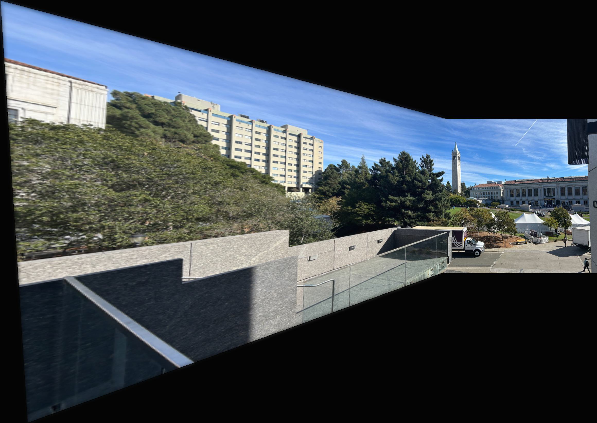
Part B: Feature Matching and Autostitching

Overview

In the second part of this project, I automated the selection of identifying potential correspondence features between two images in order to compute a homography and create our mosaic.

Harris Corner Detector

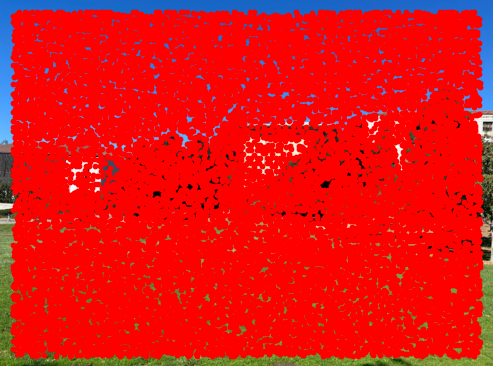
The first step in finding potential correspondence points in our images, is to think about what makes a point a good candidate to be a correspondence. Intuitively, corners in our images are good candidates due to their prominence and the ease in localizing them. This is one of the easiest ways to manually select correspondences. To automate the selection of these corners, I used a Harris corner detector. When we look at a point through a small window, if the point is a corner, when we shift this window in either the \(x\) or \(y\) direction, there should be a significant change in intensity. This results in the identification of "corners" in our image that we as humans may not think of as corners. However, this is fine as these points are still meet our criteria for a candidate correspondence.

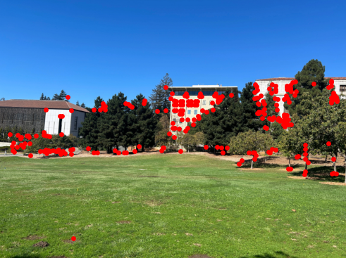
Above is the result of running the Harris corner detector on one of my sample images. Notice in the left image, that they are quite a lot of potential corners. In the right image, I displayed the 250 strongest corners as determined by the Harris corner detector's metric. So it is evident that we will need to reduce the numbeer of candidate correspondences. However, it does not seem that simply choosing the strongest Harris corners is ideal.

Adaptive Non-Maximal Suppression (ANMS)

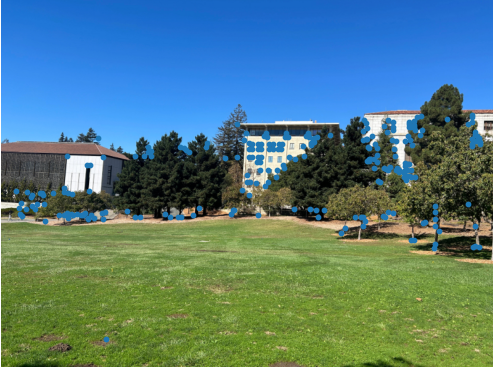
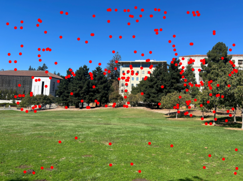
Notice that the strongest corners in our image are very clustered together and if we were to try to compute a homography using these points, it could be quite noisy. Ideally, we have correspondence points that are spread out evenly across the image. To do this, I used a technique known as Adaptive Non-Maximal Suppression (ANMS) which is described in Multi-Image Matching using Multi-Scale Oriented Patches. For each candidate point \(x_i\) we define its suppression radius: $$r_i = \min_j |x_i - x_j|, s.t. f(x_i) < c_{robust}f(x_j), x_j \in \mathcal{I}$$ where \(\mathcal{I}\) is the set of all candidate points. For this project I used \(c_{robust} = 0.9\) as suggested in the paper. Then we sort these points in order of decreasing \(r_i\) to determine the best candidate points for computing a homography. Intuitively, what we're defining as the best correspondence candidates are points that locally dominant (in terms of their Harris corner value) in the image. This in turn makes the distribution of our candidate correspondences more well-distributed throughout the image.

Below is a comparison of the 250 best candidate points as defined by using the Harris corner strength versus using ANMS:

Feature Descriptor Extraction

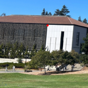
The next step after we have identified a good set of candidate correspondences, we need to automate the matching of points between the two images of interest. The first step in doing this is to define a descriptor of each of our features. I did this by first defining an axis-aligned \(40 \times 40\) pixel patch roughly centered at the point of interest. Then I downsampled this patch to an \(8 \times 8\) pixel patch (with anti-aliasing) and flattened it into a \(64\)-D vector. Then this vector was bias/gain normalized so that its elements would have \(\mu = 0\) and \(\sigma = 1\).

Below is a sample feature vector, reshaped to be \(8 \times 8\) pixels and its corresponding point on the glade image:

Feature Matching

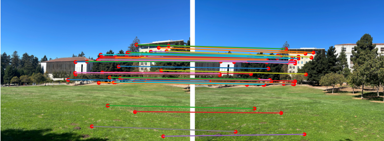
After we have defined a feature vector for each of our candidate correspondences, we can begin finding the matches. In order to do this, I first computed the distance between each candidate point's feature vector in one image to the feature vectors every candidate point in the other image. I then determine each point's nearest neighbor in the other image, creating a distance matrix. As a sanity check, I ensure symmetry of each point's nearest neighbor (i.e. if \(x_{2j}\) is the nearest neighbor of \(x_{1i}\), then \(x_{1i}\) should also be the nearest neighbor of \(x_{2j}\)).

However, instead of simply thresholding on the distance between a point and its nearest neighbor, we threshold the ratio of the distances betweeen a point's nearest neighbor and second nearest neighbor. This is known as Lowe's trick, Intuitively, if the nearest neighbor is a correct match to our point, then its feature vector must be much closer to that of our point, than the the second nearest neighbor's feature vector.

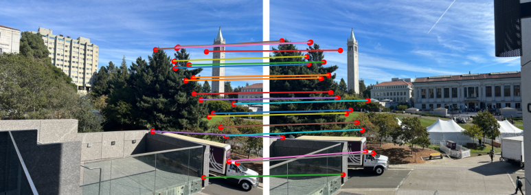
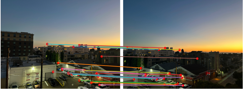
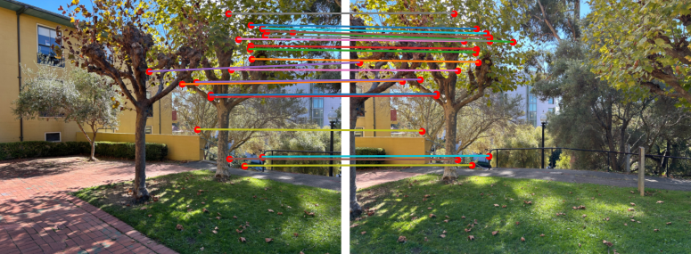
Below are subset of the points that were matched for the image pairs used to make mosaics in part A:

RANSAC

Despite our previous efforts to reject outliers, a few will still make it into our set of correspondences. It is important to not use these outliers because the Least Squares we use in our homography computation is sensitive to outliers and can significantly ruin the warping of our images. In order to mitigate this, I implemented the Random Sample Consensus (RANSAC) alogrithm to determine the points that should be used for computing the homography.

The RANSAC algorithm used followed the following steps:

1. Select 4 random correspondence pairs \((p_1, q_1), (p_2, q_2), (p_3, q_3), (p_4, q_4)\) from the matches found.
2. Compute the homography \(H\) given by these pairs of points such that \(q_i = Hp_i\)
3. Now for all of the potential correspondence pairs, determine \(||q_i - Hp_i|| < \epsilon\) for some \(\epsilon \in \mathbb{R}\). Classify the pair as an inlier if this equality holds true and as an outlier otherwise.
4. Repeat steps 1-3 until you have completed the number of iterations desired.
5. Keep the largest set of inliers
6. Re-compute the Least Squares estimate for \(H\) for all the inliers.

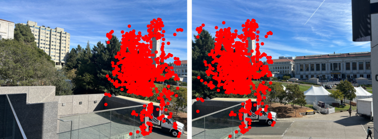
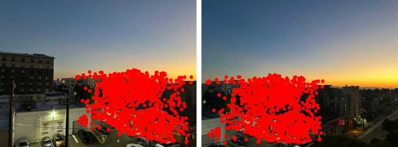
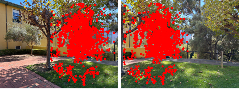
For this project I had RANSAC perform 10000 iterations and used \(\epsilon = 4\)

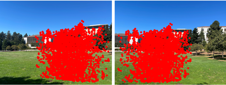
Below are displays of the a maxium set of inliers when RANSAC was peformed on the images:

Results

After computing the homography \(H\), I used the same process as described in part A to create the mosaics. Below are the moasics created from the manual correspondence selection and the automatic correspondence selection. As we can see, the automation of the feature selection does create mosaics that are just as good if not better than the mosaics created by the manually selecting correspondences.

Reflections

I learned a lot from this project. I would say the most significant thing I learned was how to autodetect features in images and match them together. The techniques and algorithms we used are things that were very unfamiliar so me to it was very cool to learn and implement them!