This project explores techniques in image processing that involve examining and analyzing an images' frequencies. Some of the techniques that are
implemented here include edge detection, blurring, sharpening, image hybridization, and image blending. Each of these techniques' implementation
will be discussed below.
Finite Difference Operator
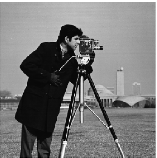
In order to create an edge detector, we first made use of the finite difference operators Dx = [1, -1] and Dy = [1, -1]T
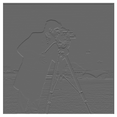
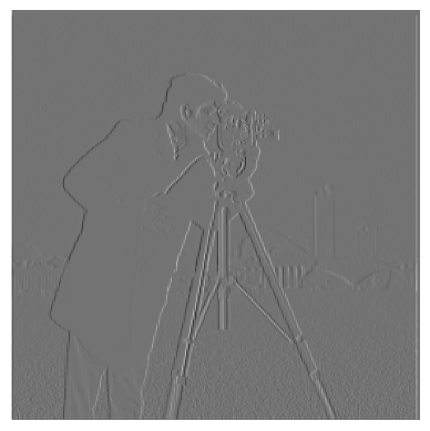
to find the partial derivatives of our image. By convolving Dx with our image, we are able to find sharp changes in pixel values of neighboring
horizontal pixels, indicating the presence of a vertical edge. Likewise, convolving Dy with our image allows us to determine the locations of
horizontal edges. These represent the partial derivatives of the images in the x and y. Then to find the edges throughout the image, we can determine the
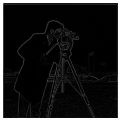
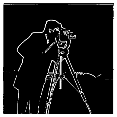
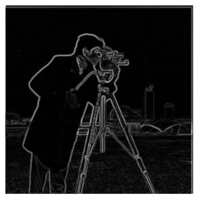
magnitude of each pixel's gradient. We do this by computing √(Dx2 + Dy2) for each pixel. Then to
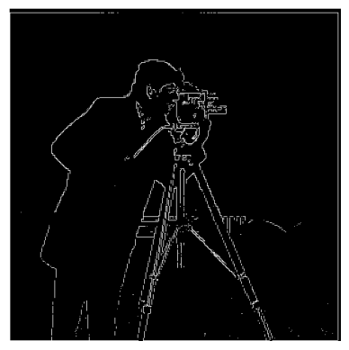
filter out noise, we binarize the image, setting a threshold for the magnitude of the gradient.
Original Cameraman Image
Dx Derivative
Dy Derivative
Gradient Magnitude
Binarized Gradient (Threshold = 60)
Derivative of Gaussian (DoG)
However, the edge image created by using the difference operators is a bit noisy. In order to produce the image above, a gradient
magnitude threshold of 60 was required and we therefore have fainter lines denoting the edges. We can improve upon this by convolving the image with a Gaussian
filter and then use our difference operators. As seen below, the derivative images are much less noisy and we can use a threshold of 20 to obtain much thicker
lines on our edge image.
Dx Derivative
Dy Derivative
Gradient Magnitude
Binarized Gradient (Threshold = 20)
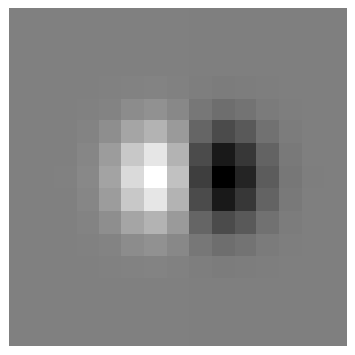
Note that we can simplify the process by first convolving our Gaussian filter with finite difference operators Dx and
Dy to get the derivative of the Gaussian kernel with respect to x and y, DoGx and DoGy. Then when
we convolve this with our camera man image, we get a nearly identical result. There are not many visible differences between the edge images
created by this and the previous method.
DoGx Derivative
DoGy Derivative
DoG Gradient Magnitude
DoG Binarized Gradient (Threshold = 20)
DoG x derivative
DoG y derivative
Image Sharpening
In this section, we implement an unsharp mask filter, which is used to artificially make an image look sharper. We go about this by
first blurring an image by a Gaussian kernel, which acts as a low pass filter. Then in order to obtain the high frequencies that were
lost, we perform a pixel-wise substraction of the blurred image from the original image. Then with this high frequency component, we
multiply it by a scaling factor α and add it back to the original image. This enhances the high frequency components of the
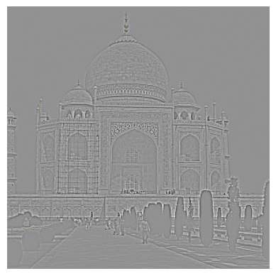
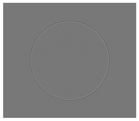
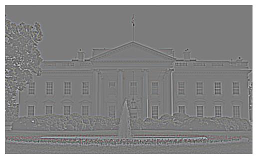
orignal image, making it appear sharper. Note that the difference images were min-max normalized for visibility purposes. Due to the
difference images containing values less than 0, the values would get clipped to 0 when displaying the image, making it very dark.
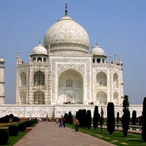
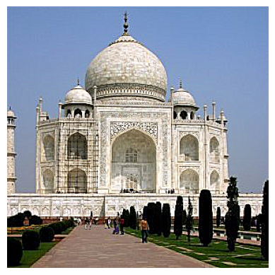
Taj Mahal
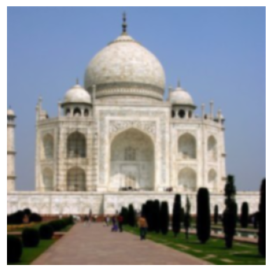
Blurred Image
Difference Image Min-Max Normalized
Sharpened Image (α = 2)
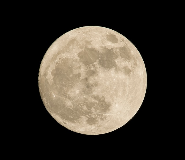
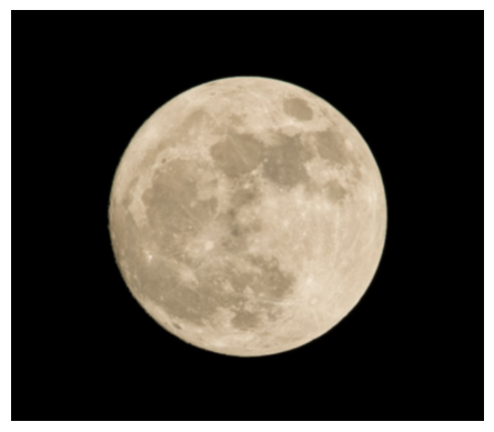
Moon
Blurred Image
Difference Image Min-Max Normalized
Sharpened Image (α = 5)
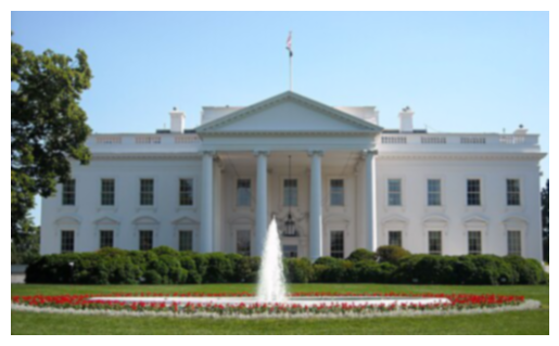
Additionally, an experiment was performed to see how well this sharpening technique could do in trying to recover lost information
due to a blur. To do this an image was blurred once, and then the above process was applied to the new blurred image (i.e. blurred again
and then substracted). As seen in the below results, this sharpening technique does do a decent job rehighlighting some features.
However, since some of the finer details were lost in the inital blurring, they were not able to be recovered in the final image.
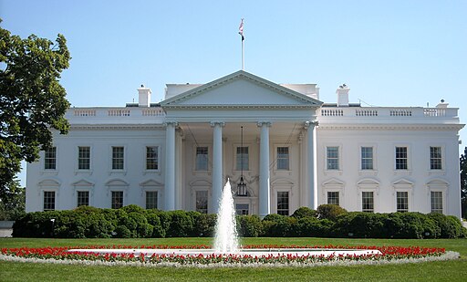
White House
Blurred Image (Base for Process)
Difference Image Min-Max Normalized
Sharpened Image (α = 3)
Hybrid Images
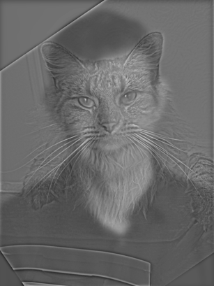
The process of creating a hybrid image entails running one image through a low pass filter and another through a high pass filter
and overlaying the two. From afar the image will look like the one passed through the low pass filter because at greater distances,
the lower frequncies of an image are more apparent. But then as you get closer to the image, it will begin to look like the one passed
through the high pass filter because the higher frequncies of the image become more apparent.
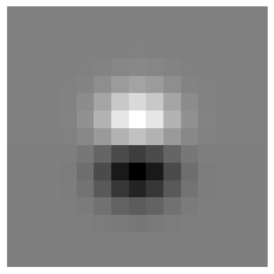
This was implemented by selecting a σ 1, a σ2, and an α. The Gaussian filter applied to the first
image meant to pass through an LPF had a kernel size of 10 * σ1 and a standard deviation of σ1. For the
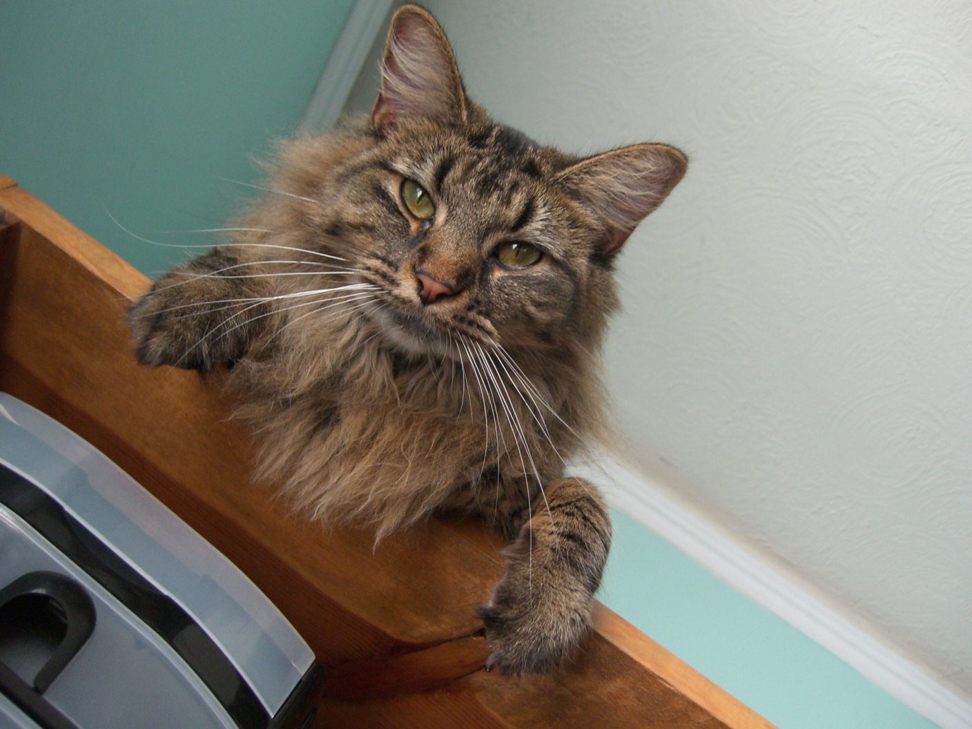
second image, its high frequency components were extracted in the same manner as done in the previous part for the image sharpening technique
(original_img - blurred_img) = hi_freq_im. The Gaussian filter used for this image had a kernel size of 10 * σ2 and a
standard deviation of σ2. Then α was used to compute a multiplier for the high frequency image when adding the two
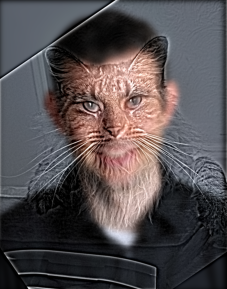
together. For gray-scale images, the two images were averaged so the image did not appear too dark. For color images, this process was applied
to each of the low pass image's RBG channels and were combined with the gray version of the high pass filter. This method seemed to get the best
qualitative results out of the possible combinations of color selection. However, when the colors of the two images did not match, this was
apparent.
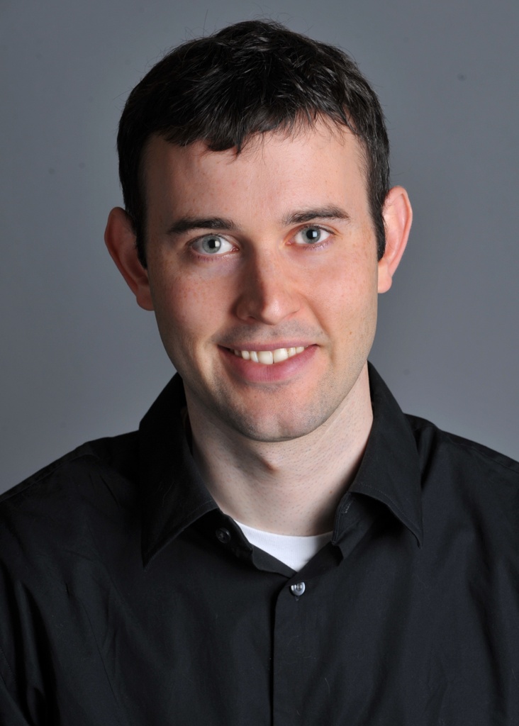
Derek and Nutmeg (Success)
Low Freq Img: Derek (σ1 = 9)
High Freq Img: Nutmeg (σ2 = 5)
Hybrid Image Gray (α = 2.5)
Hybrid Image Color (α = 2.5)
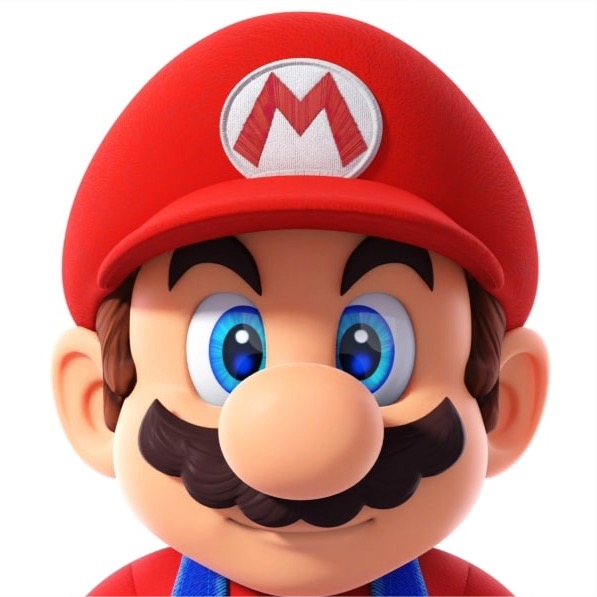
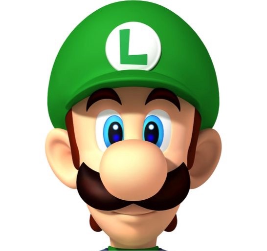
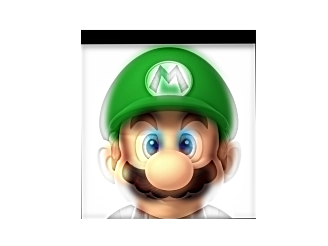
Mario Bros. (Success)
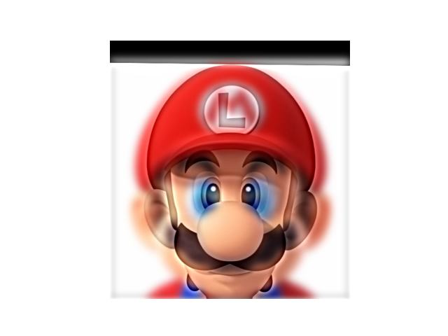
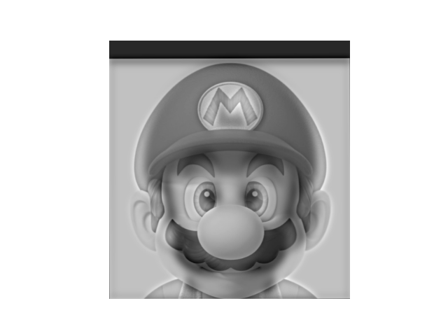
Low Freq Img: Mario (σ1 = 8)
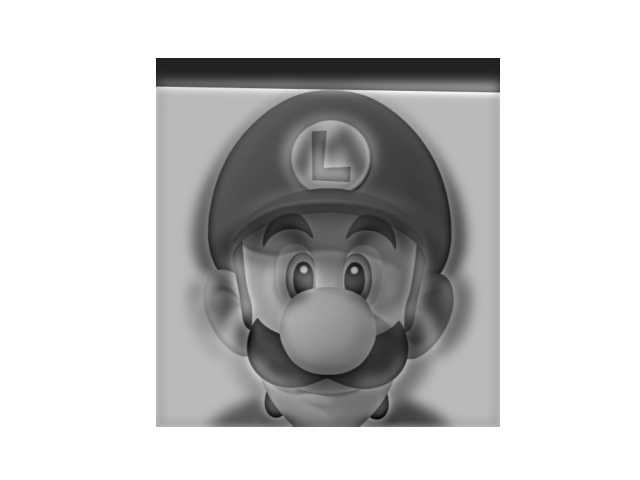
High Freq Img: Luigi (σ2 = 6)
Hybrid Image Gray (α = 1)
Hybrid Image Color (α = 1)
Low Freq Img: Luigi (σ1 = 8)
High Freq Img: Mario (σ2 = 6)
Hybrid Image Gray (α = 1)
Hybrid Image Color (α = 1)
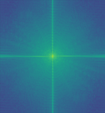
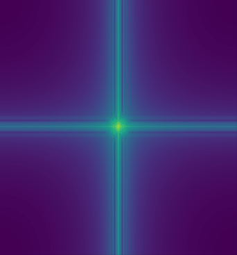
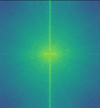
This result was my favorite so a Fourier analysis was additionally performed on each of these images. The original images' Fourier transfrom
was visualized before and after filtering, and then finally once they were combined. This Fourier analysis is for the hybrid image composed of
the low frequency Mario and the high frequency Luigi.
Low Freq Img: Mario (Original)
Low Freq Img: Mario (Filtered)
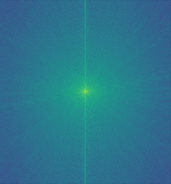
High Freq Img: Luigi (Original)
High Freq Img: Luigi (Filtered)
Hybrid Image
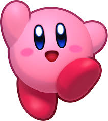
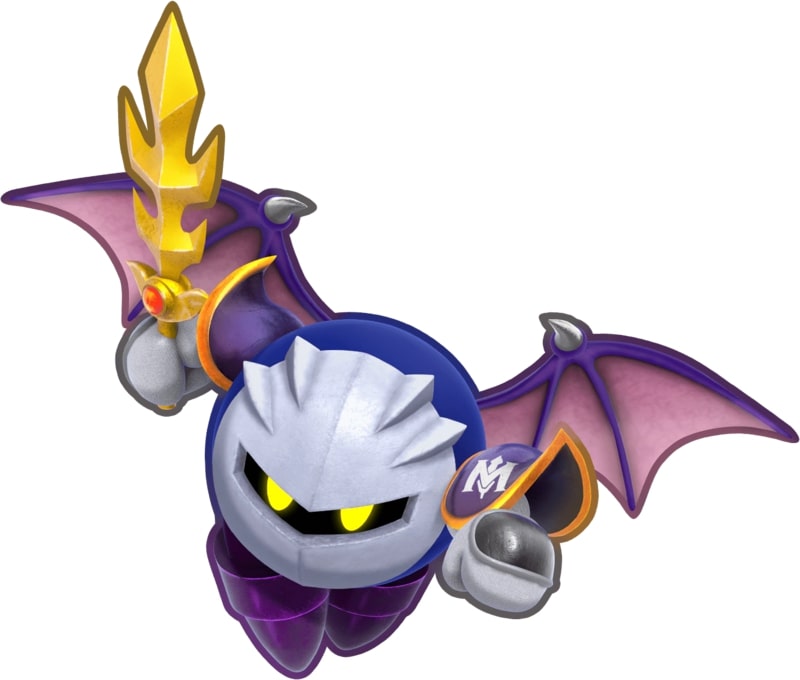
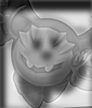
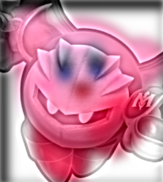
Kirby & Meta Knight (Partial Failure)
This hybrid is deemed as a partial failure because while the gray-scale hybrid image works pretty well, the color hybrid does not.
Kirby's pink color is too prominent so Meta Knight's high frequencies are not as apparent even close up.
Low Freq Img: Kirby (σ1 = 7)
High Freq Img: Meta Knight (σ2 = 4)
Hybrid Image Gray (α = .5)
Hybrid Image Color (α = 1)
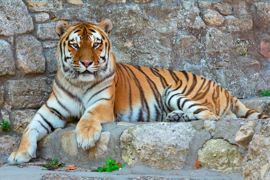
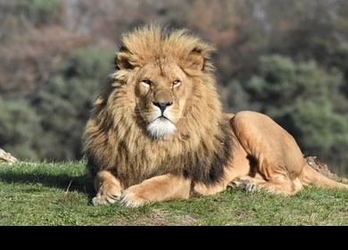
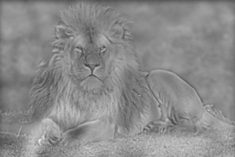
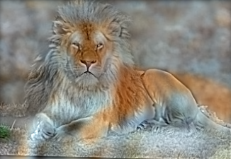
Lion & Tiger (Failure)
This hybrid is deemed as a failure because the color and gray-scale hybrid images only worked decently for one of the images.
In the color hybrid, the low frequency tiger relies too much on its color to be made out from afar. In the gray-scale image, the
patterns on the tiger blend too much with the background of the image so it is difficult to distinguish. Additionally, in the colored
image, the high frequency lion is too difficult to make out with the color of the tiger dominating the image.
Low Freq Img: Tiger (σ1 = 5)
High Freq Img: Lion (σ2 = 2)
Hybrid Image Gray (α = 1.2)
Hybrid Image Color (α = 1.2)
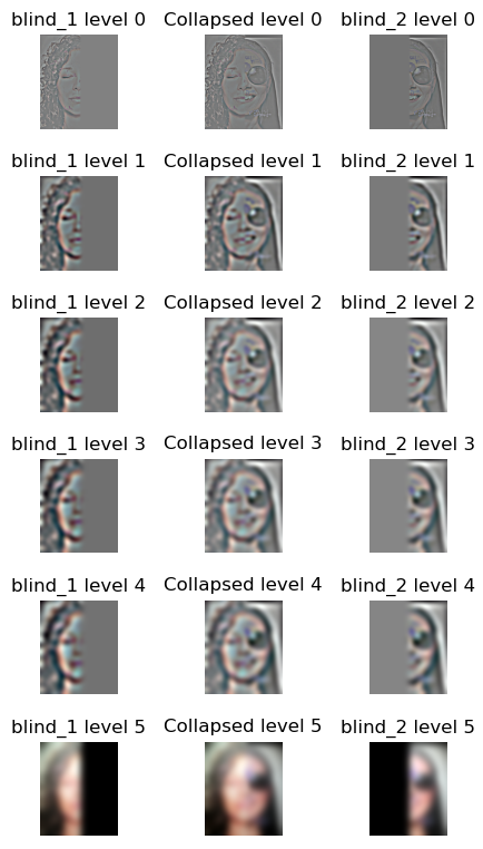
Gaussian and Laplacian Stacks
A Gaussian stack is created by repeatedly blurring an image with a Guassian kernel without downsampling so the image at each level of
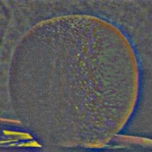
the stack will be the same size. From here a Laplacian stack can be created by substracting images in the Guassian stack. For example,
the level 0 Laplcian stack is computed by Gaussian level 0 minus Gaussian level 1. Then the final image in the Laplacian stack is the
same as the last image in the Gaussian stack. Note that the images in the Laplacian stack below have been min-max normalized for purposes of
display.
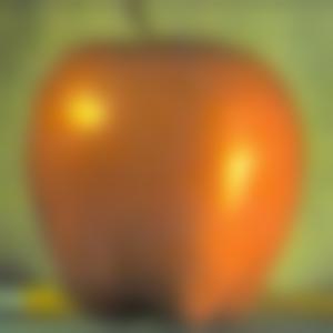
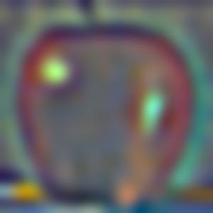
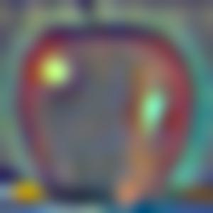
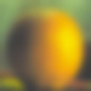
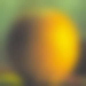
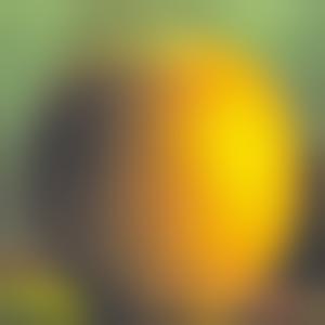
Apple: Gaussian Level 0
Apple: Gaussian Level 1
Apple: Gaussian Level 2
Apple: Gaussian Level 3
Apple: Gaussian Level 4
Apple: Gaussian Level 5
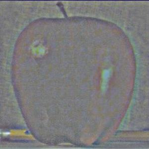
Apple: Laplacian Level 0
Apple: Laplacian Level 1
Apple: Laplacian Level 2
Apple: Laplacian Level 3
Apple: Laplacian Level 4
Apple: Laplacian Level 5
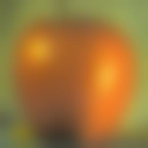
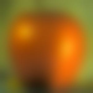
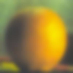
Orange: Gaussian Level 0
Orange: Gaussian Level 1
Orange: Gaussian Level 2
Orange: Gaussian Level 3
Orange: Gaussian Level 4
Orange: Gaussian Level 5
Orange: Laplacian Level 0
Orange: Laplacian Level 1
Orange: Laplacian Level 2
Orange: Laplacian Level 3
Orange: Laplacian Level 4
Orange: Laplacian Level 5
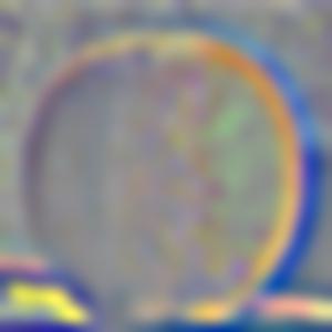
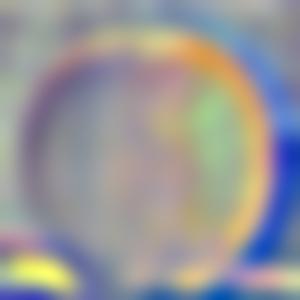
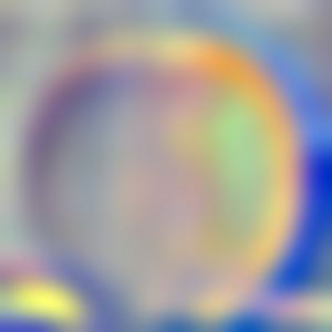
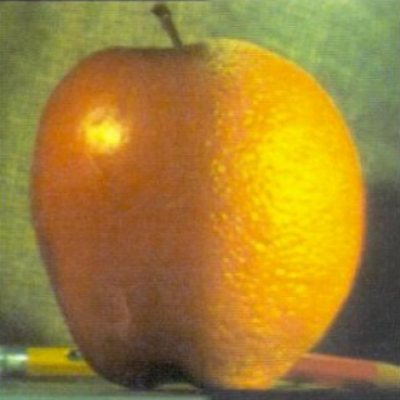
Multiresolution Blending
The cool thing about Laplacian stacks is that we can use them for multiresolution blending of two images. The famous example of this is
the orapple, an image that is left half apple and right half orange, and the boundary between the two is blended quite nicely. This is done
by performing a blending on pairs of images from each Laplacian stack. This is done because features of different frequencies require a
different blurred mask in order for the features to appear smoothly. So by creating Laplacian stacks of both images, we effectively perform
a band pass filtration and can blend each frequency range independently. Then afterward we can collapse the blended images back into a single
blended image. For gray-scale images this is simply done on the single channel. For color images, this is done individually for each of the
RGB channels at each layer. The Gaussian kernel used to generate the stacks is of size 5 * σ with a standard deviation of σ.
Additionally, N is defined as the max level of the Gaussian/Laplacian stacks.
The creation of the masks for this blending can be done by creating a Gaussian stack of an initial mask. For the following two sets of blending,
an initial mask was created in the size of the images such that the left half of the mask was all 1s (white) and the left half was all 0s (black).
Then the same Gaussian that was used the blur the images that we are blending was used to blur the mask. Then each level of the mask's Gaussian
stack was applied to the images on the same level in the Laplacian stack. At each level, the combined image was computed with the following:
combined_img = mask * left_img + (1 - mask) * right_img.
Mask Level 0
Mask Level 1
Mask Level 2
Mask Level 3
Mask Level 4
Mask Level 5
Orapple
Apple (Left)
Orange (Right)
Blended (N = 5, σ = 8)
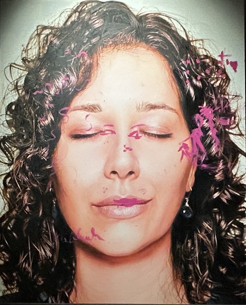
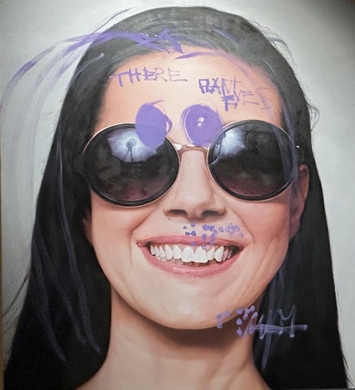
Blind Artists
Below is a combination of pictures of two paintings I viewed in an art gallery in New York in the summer of 2024. For context, an artist painted
hyper-realistic portraits of people who have been blind since birth. Then afterward the subjects were instructed to paint over the painting with
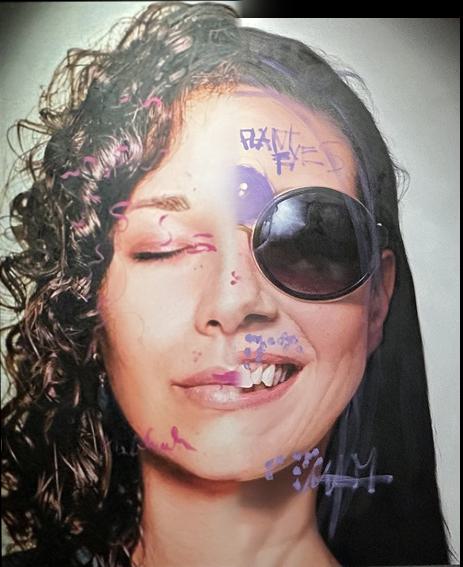
their interpretation of themselves. Overall I think this blending was successful. There are a couple inconsistencies with the mouths and the tops
of the paintings due to alignment of the picutres, but most of it is blended very smoothly.
Left Painting
Right Painting
Blended (N = 5, σ = 10)
Blind Art Laplacian Stacks
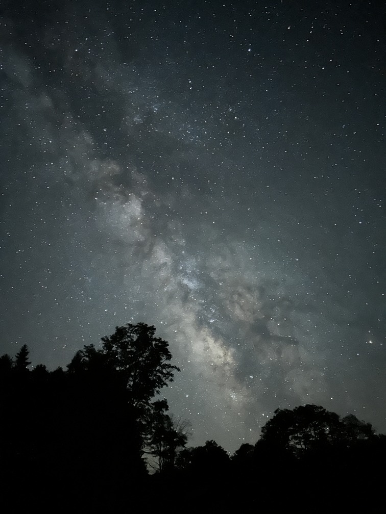
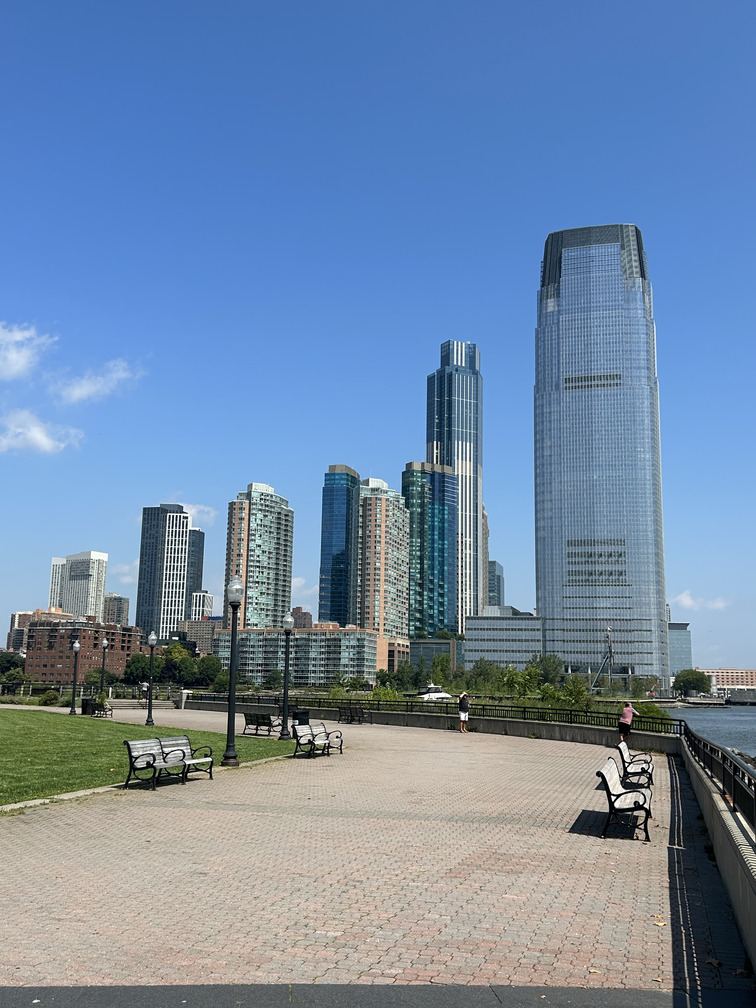
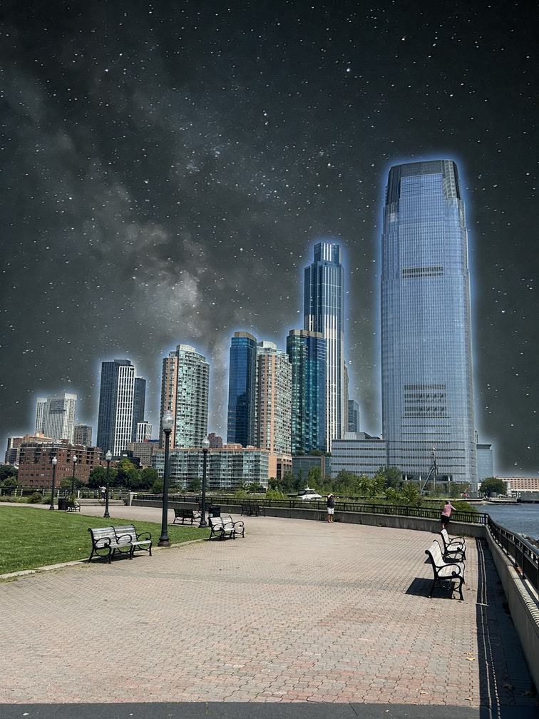
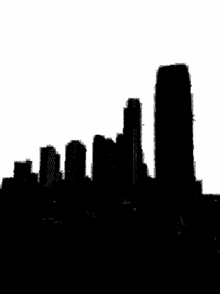
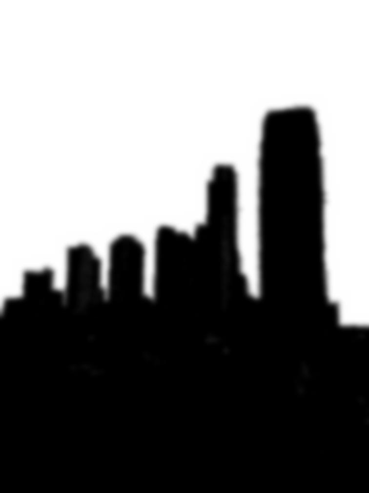
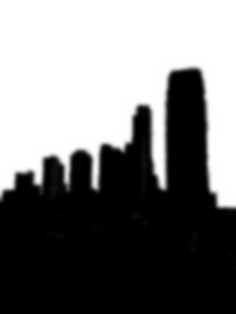
Milky New York (Irregular Mask)
Below is a combination of two pictures I took in the summer of 2024. One is a picture of the Milky Way view from Cherry Springs State Park
in Pennsylvania. The other picture is of some buildings in New York City. I created a custom mask (a bit poorly) that would remove the sky
of the New York picture and replace it with the sky of the Milky Way picture. My mask was not perfect and as a result the color of the blue
sky was not entirely removed. But it ended creating a nice effect of a blue glow around the buildings.