For this final project, I completed two separate projects of my choice. Both projects are displayed below on this webpage.
Project 1: Gradient Domain Fusion
Overview
Previously, I have done image blending by using Gaussian and Laplacian stacks to blend different frequencies of images independently. This overall does result in a smooth transition from one image to another, however it is not the best tool for editing in images in a photo-realistic manner. This is especially true when the colors of the iamges are not similar.
In an attempt to remedy this, I implement Poisson blending. Since our eyes are more sensitive to an image's gradient than to the overall pixel intensity, we can modify the intensity of the pixels in the source image to closely match the gradients of the target image. We can do this by setting up the following least squares optimization problem: $$\vec{v} = \underset{\vec{v}}{\arg\min} \sum_{i \in S, j \in N_i \cap S} ( (v_i - v_j) - (s_i - s_j) )^2 + \sum_{i \in S, j \in N_i \cap \neg S} ( (v_i - t_j) - (s_i - s_j) )^2 $$ Note that the above equation has some redundant terms, which is not accurate. It is written this way for simplicity. All differences are weighted equally in this optimization
In the interior of our source image, for each pixel \(i\) and each pixel \(j\) in the 4-neighborhood around \(i\), we want to minimize the sum of squared differences between gradient of the new pixels' insensity \(v_i - v_j\) and the gradient of the source image's pixel insentiy \(s_i - s_j\). For the pixels along the border of our source image we minimize the sum of squared differences between \(v_i - t_j\) and \(s_i - s_j\), where \(t_j\) is a pixel on our target image. This optimization ensures that the gradients of our new pixels match closely to that of the source image. To solve this least squares problem, we set up the system \(A\vec{v} = \vec{b}\), where \(A\) is a sparse matrix, and solve for the optimal solution \(\vec{v}^* = (A^TA)^{-1}A^T \hspace{1pt}\vec{b}\). After this, the elements of vector \(\vec{v}^*\) are assigned accordingly to the pixels in our blended image.
Toy Problem
While implementing the above process is not too difficult, it is easy to make mistakes, especially in the creation of \(A\) and \(\vec{b}\). So, I first tested this algorithm on a toy problem, in which I simply reconstructed an image instead of blending one image into another. Note that since there is no target image, no equations from the second summation above were included here. This also required me add another contraint, \(v(0,0) = s(0,0)\). This sets that the top left corner of our new image to have the same pixel value as the source image. This was done because without this constraint, there would be multiple sets of pixel insenties that would be valid. Adding this constraint, our reconstruction becomes perfect. Below is the result of this process.

|
|
Poisson Blending
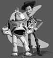
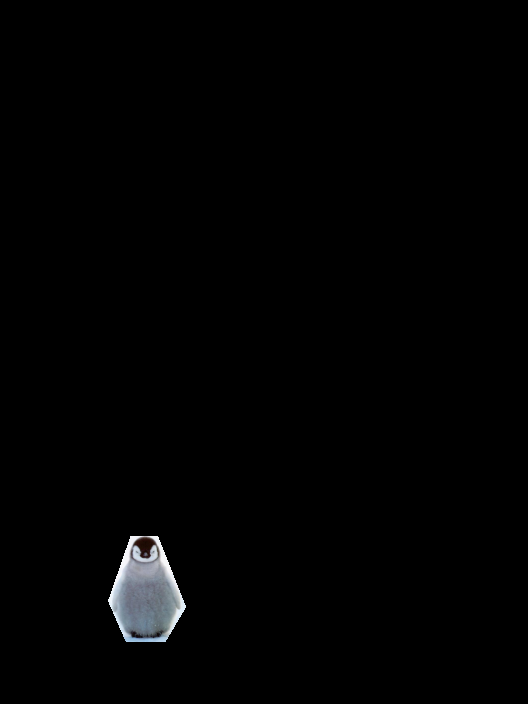
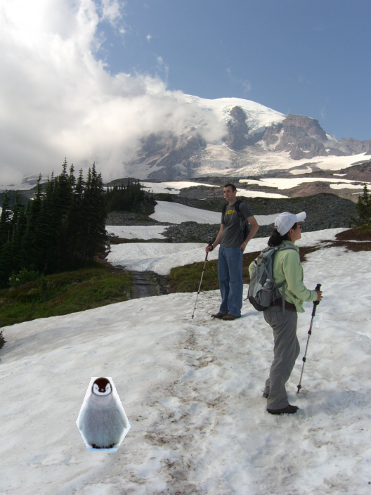
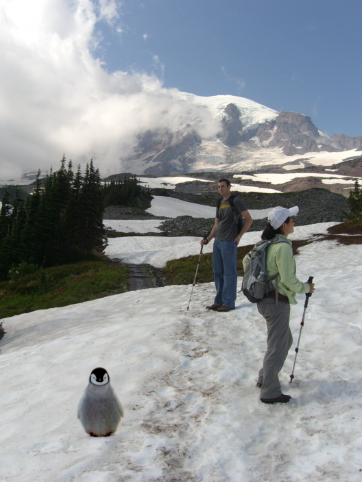
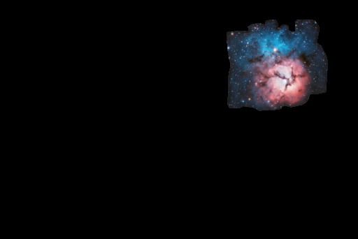
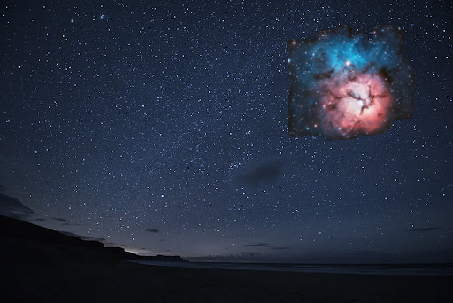
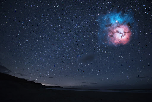
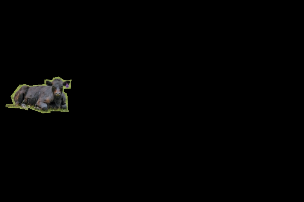
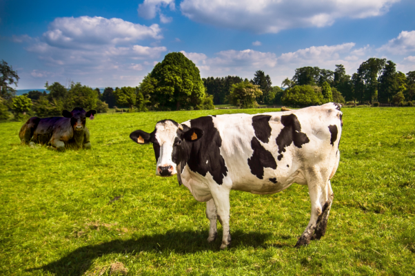
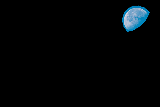
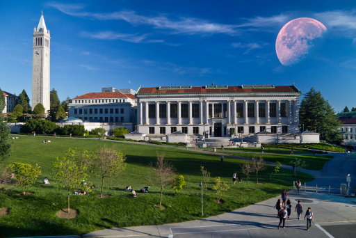
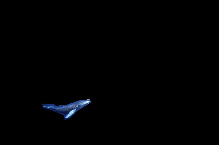
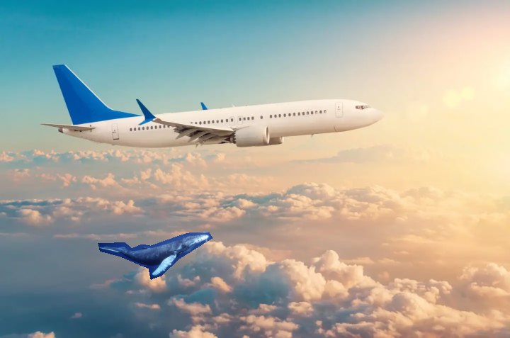
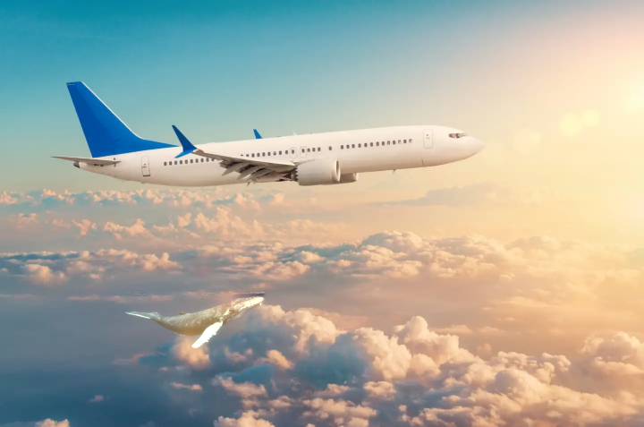
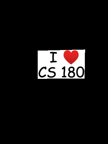
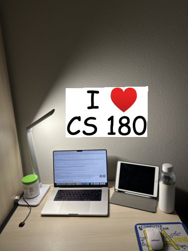
To perform Poisson blending, I first had to create a mask around the relevant pixels in the source image and choose a location to place them in the target image. After this, I simply set up the above least squares optimization problem as is into the system \(A\vec{v} = \vec{b}\) for each color channel and solved for each color's \(\vec{v}^*\). After doing this, I set the desired pixel values in the target image to the corresponding elements in \(\vec{v}^*\). Below are some results of this process. I include images of the source image mask, an initial replacement of pixels in the target image, and the output of the Poisson blending.
Results
|
|
|
|
|
|
|
|
|
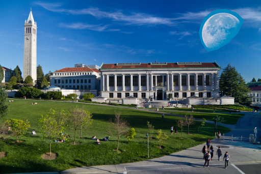
The three blendings above were overall quite good. Aside from discrepencies such as relative size of objects and abscence of shadows, it seems like the source images are a part of the target image. In each of these situations, the color of objects did change slightly, but these changes aren't very obvious in the final images and are reasonable given the difference in lighting.
Failures (Depending on Your Opinion)
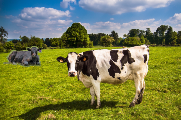
Below are some image blends that did ultimately change the color of the source too much to seem realistic. However in the images below, I think these color changes ended up being pretty cool.
|
|
|
|
|
|
Bells and Whistles: Mixed Gradients
As an extension to Poisson blending I implented a mixed gradients method, in which the optimization problem was modified to be the following: $$\vec{v} = \underset{\vec{v}}{\arg\min} \sum_{i \in S, j \in N_i \cap S} ( (v_i - v_j) - d_{ij} )^2 + \sum_{i \in S, j \in N_i \cap \neg S} ( (v_i - t_j) - d_{ij} )^2 $$ where \(d_{ij} = s_i - s_j\) if \(|s_i - s_j| \geq |t_i - t_j|\) and \(d_{ij} = t_i - j_j\) if \(|t_i - t_j| \lt |s_i - s_j|\)
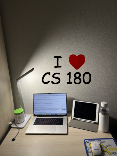
This change makes it so that we compare the gradient of our new pixel to the gradient of the source or target image, depending on which one has the greater magnitude. Then just like for Poisson, we solve a least squares system. This process is very good at blending images onto textured surfaces. Below are some results of this process. My favorite image is the shirt, because you can really see the texture and folds of the shirt in the new image. It makes it look like the logo is actually on the shirt.
|
|
|
|
|
|
|